Final Project: Electric Rickshaw modelling

Q) 

Create a detailed MATLAB model of an electric rickshaw (three wheel passenger vehicle) as per details below: 

Rear wheels driven by PM brushed type motor

Assume efficiency points of motor controller and motor

Make an excel sheet of all input and assumed data 

Results: For any three standard driving cycles show energy consumption, temperature rise of motor and controller for 100 km constant speed driving at 45 kmph.

Ans:

Aim:

Create a detailed MATLAB model of an electric rickshaw (three wheel passenger vehicle) as per details below: 

Rear wheels driven by PM brushed type motor

Assume efficiency points of motor controller and motor

Make an excel sheet of all input and assumed data 

What is an Electric Rickshaw:

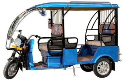
Electric rickshaws have been becoming more popular in some cities since 2008 as an alternative to auto rickshaws and pulled rickshaws because of their low fuel cost, and less human effort compared to pulled rickshaws. They are being widely accepted as an alternative to petrol/diesel/CNG auto rickshaws. They are three-wheelers powered by an electric motor ranging from 650 to 1400  Watts. They are mostly manufactured in India and China, only a few other countries manufacture these vehicles. Battery-run rickshaws could be a low-emitter complementary transport for the low-income people, who suffer most from a lack of transport facility, if introduced in a systematic manner according to experts.

Design and Construction:

These rickshaws have a M.S(Mild Steel) tubular Chassis, consisting of three wheels with a differential mechanism at the rear wheels. The motor is brushless DC motor manufactured mostly in India and China. The electrical system used in Indian version is 48V and Bangladesh is 60V. The body design from most popular Chinese version is of very thin iron or aluminum sheets. Vehicles made in fiber are also popular because of their strength and durability, resulting in low maintenance, especially in India. Body design is varied from load carriers, passenger vehicles with no roof, to full body with windshield for drivers comfort. It consist of a controller unit.They are sold on the basis of voltage supplied and current output, also the number of mosfet (metal oxide field effect transistors) used. The battery used is mostly lead acid battery with life of 6–12 months. Deep cycle batteries designed for electric vehicles are rarely used. Weight of the electric car has also been a recurring design difficulty in them.

Block Diagram:

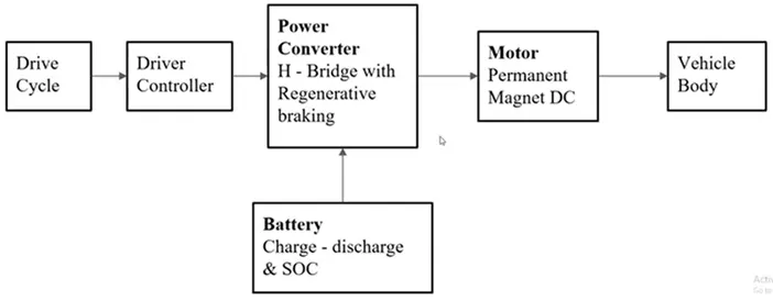
In an Electric Rickshaw the main blocks are

Drive cycle: A driving cycle is a series of data points representing the speed of a vehicle versus time. Driving cycles are produced by different countries and organizations to assess the performance of vehicles in various ways, as for instance fuel consumption, electric vehicle autonomy and polluting emissions.

Driver controller: The controller transforms the batteries direct current into alternating current (for AC motors only) and regulates the energy flow from the battery. ... In the early electric vehicles with DC motors, a simple variable-resistor-type controller controlled the acceleration and speed of the vehicle.

Power converter: In electric engineering, a DC to DC converter is a category of power converters and it is an electric circuit which converts a source of direct current (DC) from one voltage level to another, by storing the input energy temporarily and then releasing that energy to the output at a different voltage.

Motor: Today, majority of the electric cars are utilizing DC motors (4 kW and less power). Induction Motor is an exceptionally well known AC motor. A considerable lot of the advanced power EV (more than 5kW), utilize Induction Motors.

Battery: Most plug-in hybrids and all-electric vehicles use lithium-ion batteries like these. Energy storage systems, usually batteries, are essential for hybrid electric vehicles (HEVs), plug-in hybrid electric vehicles (PHEVs), and all-electric vehicles (EVs).

Vehicle body: Car bodies are most often made of steel, which is strong and durable, but also pretty heavy—especially for electric power to move on its own.

Simulink model:

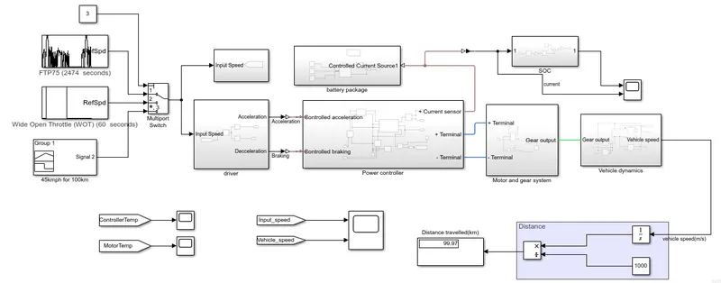
Components used: 

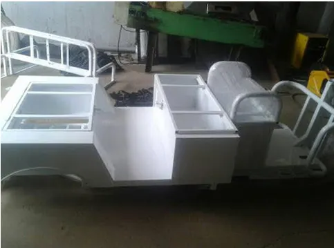
Vehicle body and wheel: 

 

 

Tire (magic Formula): 

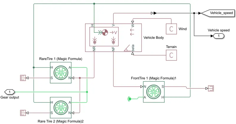
Represents the longitudinal behavior of a highway tire characterized by the tire Magic Formula. The block is built from Tire-Road Interaction (Magic Formula) and Simscape Foundation Library Wheel and Axle blocks. Optionally, the effects of tire inertia, stiffness, and damping can be included.

A is the mechanical rotational conserving port for the wheel axle

H is the mechanical translational conserving port for the wheel hub through which the thrust developed by the tire is applied to the vehicle.

N is a physical signal input port that applies the normal force acting on the tire.

S is a physical signal output port that reports the tire slip.

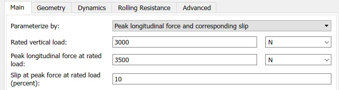
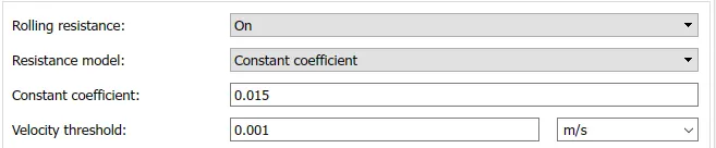
Specification of Tire:

Vehicle body:

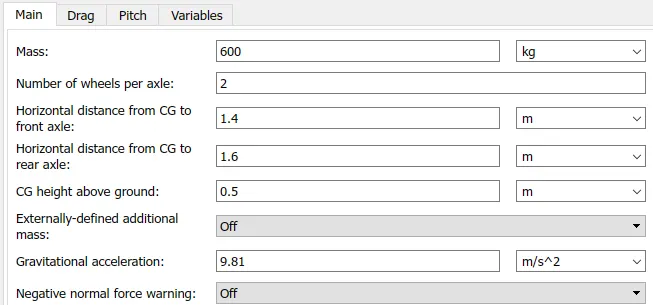
Represents a two-axle vehicle body in longitudinal motion. The block accounts for body mass, aerodynamic drag, road incline, and weight distribution between axles due to acceleration and road profile. The vehicle can have the same or a different number of wheels on each axle. Optionally include pitch and suspension dynamics or additional variable mass and inertia.

H is the mechanical translational conserving port associated with the horizontal motion of the vehicle body. The resulting traction motion developed by tires should be connected to this port.

V, NF, and NR are physical signal output ports for vehicle velocity and front and rear normal wheel forces, respectively.

W and beta are physical signal input ports corresponding to headwind speed and road inclination angle, respectively.

Specification of Vehicle body:

PS Constant:

This block creates a physical signal constant:

y = constant

The Constant parameter accepts both positive and negative values. The block output is a physical signal port.

This PS constant is connected to the Vehicle body port W and delt for we can change the value of angel and wind velocity but we kept this value now one.

Gear Box:

The block represents an ideal, non-planetary, fixed gear ratio gear box. The gear box is characterized by its only parameter, Gear ratio, which can be positive or negative. Connections S and O are mechanical rotational conserving ports associated with the box input and output shaft, respectively. The gear ratio is determined as the ratio of the input shaft angular velocity to that of the output shaft.

The block generates torque in positive direction if a positive torque is applied to the input shaft and the ratio is assigned a positive value.

DC Motor:

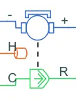
This block represents the electrical and torque characteristics of a DC motor. The block assumes that no electromagnetic energy is lost, and hence the back-emf and torque constants have the same numerical value when in SI units. Motor parameters can either be specified directly, or derived from no-load speed and stall torque. If no information is available on armature inductance, this parameter can be set to some small non-zero value.

When a positive current flows from the electrical + to - ports, a positive torque acts from the mechanical C to R ports. Motor torque direction can be changed by altering the sign of the back-emf or torque constants.

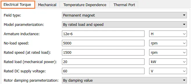
Specification of DC Motor:

Thermal Port:

The block has an optional thermal port, hidden by default. To expose the thermal port, right-click the block in your model, and then from the context menu select Simscape > Block choices > Show thermal port. This action displays the thermal port H on the block icon, and exposes the Temperature Dependence and Thermal Port parameters.

Use the thermal port to simulate the effects of copper resistance losses that convert electrical power to heat. For more information on using thermal ports and on the Temperature Dependence and Thermal Port parameter.

Temperature Sensor:

This block measures temperature in a thermal network. There is no heat flow through the sensor. The physical signal port T reports the temperature difference across the sensor. The measurement is positive when the temperature at port A is greater than the temperature at port B.

DC Motor Controller:

H Bridge:

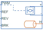
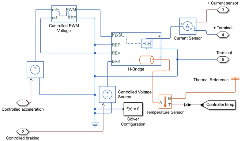
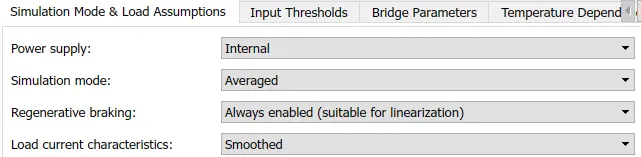
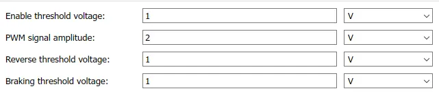
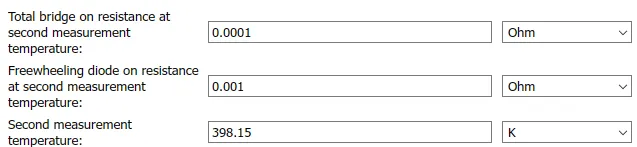
This block represents an H-bridge motor drive. The block can be driven by the Controlled PWM Voltage block in PWM or Averaged mode. In PWM mode, the motor is powered if the PWM port voltage is above the Enable threshold voltage. In Averaged mode, the PWM port voltage divided by the PWM signal amplitude parameter defines the ratio of the on-time to the PWM period. Using this ratio and assumptions about the load, the block applies an average voltage to the load that achieves the correct average load current. The Simulation mode parameter value must be the same for the Controlled PWM Voltage and H-Bridge blocks.

If the REV port voltage is greater than the Reverse threshold voltage, then the output voltage polarity is reversed. If the BRK port voltage is greater than the Braking threshold voltage, then the output terminals are short circuited via one bridge arm in series with the parallel combination of a second bridge arm and a freewheeling diode. Voltages at ports PWM, REV and BRK are defined relative to the REF port.

If exposing the power supply connections, the block only supports PWM mode.

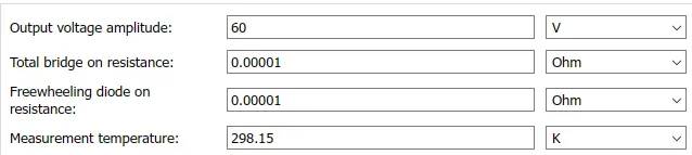
Specification of H-bridge:

Controlled PWM Voltage:

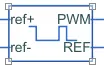
This block creates a Pulse-Width Modulated (PWM) voltage across the PWM and REF ports. The output voltage is zero when the pulse is low, and is equal to the Output voltage amplitude parameter when high. Duty cycle is set by the input value. Right-click the block and select Simscape->Block choices to switch between electrical +ref/-ref ports and PS input u to specify the input value.

At time zero, the pulse is initialized as high unless the duty cycle is set to zero or the Pulse delay time is greater than zero.

The Simulation mode can be set to PWM or Averaged. In PWM mode, the output is a PWM signal. In Averaged mode, the output is constant with value equal to the averaged PWM signal.

Specification of PWM voltage:

Controlled voltage source:

The block represents an ideal voltage source that is powerful enough to maintain the specified voltage at its output regardless of the current passing through it. The output voltage is V = Vs, where Vs is the numerical value presented at the physical signal port.

Current Sensor:

The block represents an ideal current sensor, that is, a device that converts current measured in any electrical branch into a physical signal proportional to the current.

Connections + and - are conserving electrical ports through which the sensor is inserted into the circuit. Connection I is a physical signal port that outputs current value.

Electrical reference:

Electrical reference port. A model must contain at least one electrical reference port (electrical ground).

Solver Configuration:

Each physical network represented by a connected Simscape™ block diagram requires solver settings information for simulation. The Solver Configuration block specifies the solver parameters that your model needs before you can begin simulation.

Each topologically distinct Simscape block diagram requires exactly one Solver Configuration block to be connected to it.

Mechanical rotational reference:

This block represents a mechanical rotational reference point, that is, a frame or a ground. Use it to connect mechanical rotational ports that are rigidly affixed to the frame (ground).

Battery Package:

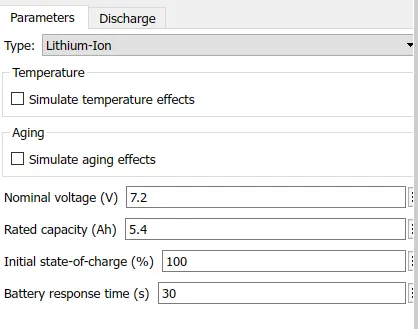
Battery system:

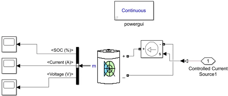
Implements a generic battery model for most popular battery types. Temperature and aging (due to cycling) effects can be specified for Lithium-Ion battery type.

Type and Specifications:

Controlled current source:

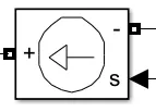
Converts the Simulink input signal into an equivalent current source. The generated current is driven by the input signal of the block.

You can initialize your circuit with a specific AC or DC current. If you want to start the simulation in steady-state, the block input must be connected to a signal starting as a sinusoidal or DC waveform corresponding to the initial values.

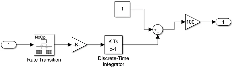
State of Charge:

Descrete-time Integrator:

This block can integrate or accumulate a signal using a forward Euler, backward Euler, or trapezoidal method. Assume that u is the input, y is the output, and x is the state. For a given step n, Simulink updates y(n) and x(n+1). In integration mode, T is the block sample time (delta T in the case of triggered sample time). In accumulation mode, T = 1. The block sample time determines when the output is computed but not the output value. K is the gain value. Values clip according to upper or lower limits.

Gain:

The Gain block multiplies the input by a constant value (gain). The input and the gain can each be a scalar, vector, or matrix.

Gain is converted from doubles to the data type specified in the block mask offline using round-to-nearest and saturation. The input and gain are then multiplied, and the result is converted to the output data type using the specified rounding and overflow modes.

Rate Transition:

The Rate Transition block transfers data from the output of a block operating at one rate to the input of a block operating at a different rate. Use the block parameters to trade data integrity and deterministic transfer for faster response or lower memory requirements. To learn about data integrity and deterministic data transfer, see Data Transfer Problems (Simulink Coder).

Powergui:

The powergui block also opens tools for steady-state and simulation results analysis and for advanced parameter design. You need the powergui block to simulate any Simulink model containing Simscape™ Electrical™ Specialized Power Systems blocks. It stores the equivalent Simulink circuit that represents the state-space equations of the model.

When using one powergui block in a model:

The powergui block becomes disabled during model update. To ensure proper model execution, do not restore the library link for the powergui block.

Driver:

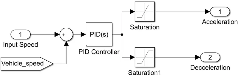
Saturation:

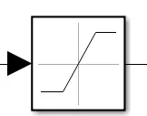
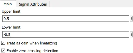
Limit input signal to the upper and lower saturation values.

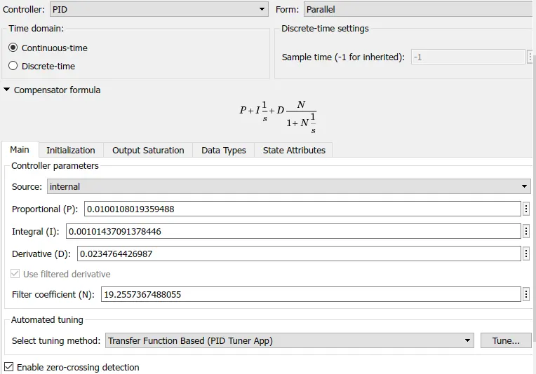
PID Controller:

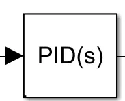
This block implements continuous- and discrete-time PID control algorithms and includes advanced features such as anti-windup, external reset, and signal tracking. You can tune the PID gains automatically using the 'Tune...' button (requires Simulink Control Design).

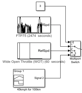
Inputs and Multiport switch:

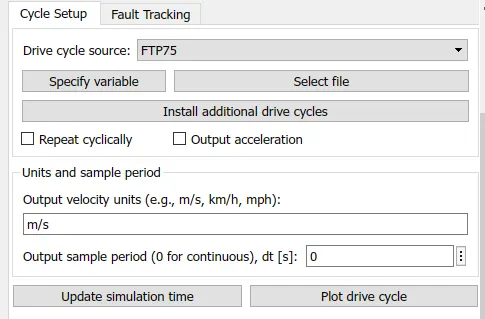
FTP75 drive cycle:

The Drive Cycle Source block generates a standard or user-specified longitudinal drive cycle. The block output is the specified vehicle longitudinal speed, which you can use to:

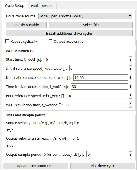
Wide Open Throttle drive cycle:

Signal Builder:

The Signal Builder block allows you to create interchangeable groups of piecewise linear signal sources and use them in a model. You can quickly switch the signal groups into and out of a model to facilitate testing. In the Signal Builder window, create signals and define the output waveforms.To open the window, double-click the block.

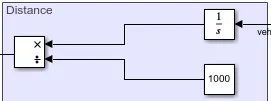
Distance calculation from vehicle speed:

Results:

(i) Using FTP75 drive cycle without tuned PID gain values:

P=1 I=1 D=0.5

Input speed vs Vehicle speed:

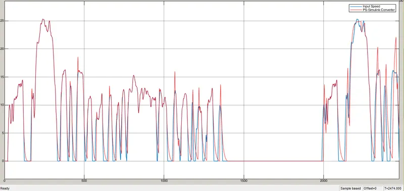
Here we can seen that input speed and vehicle speed are almost overlapped this shows us that vehicle speed following the input speed. 

Battery SOC and Current:

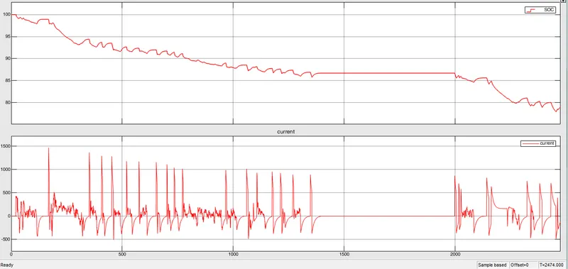
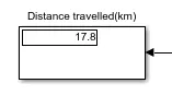
The above graph shows that remaining charge in the battery in terms of percentage after covering 17.76km of distance.

Controller Temperature:

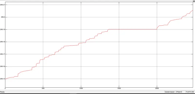
As we already know as vehicle starts to running then temperature also increases in motor controller division.

Motor Temperature:

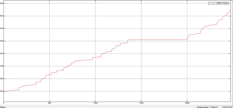
This scope result shows temperature of motor, if we again modified the pid gain values then motor temperature goes slightly reduces. here we can see that without pid gain values the temperature of motor reaches nearly 600K.

(ii) Using FTP75 drive cycle with tuned PID gain values:

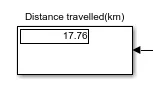
In this model we already tune the pid gain values hence we are getting 17.76km distance for FTP75 drive cycle.

Input speed vs Vehicle speed:

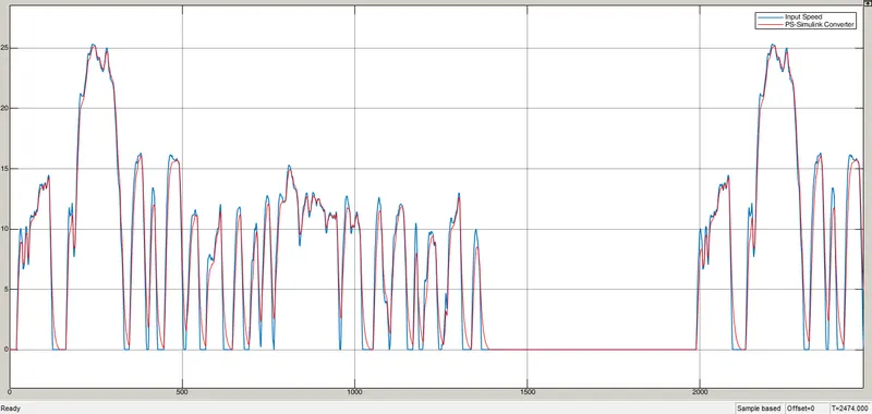
Here we can seen that input speed and vehicle speed are almost overlapped this shows us that vehicle speed following the input speed. 

Battery SOC and Current:

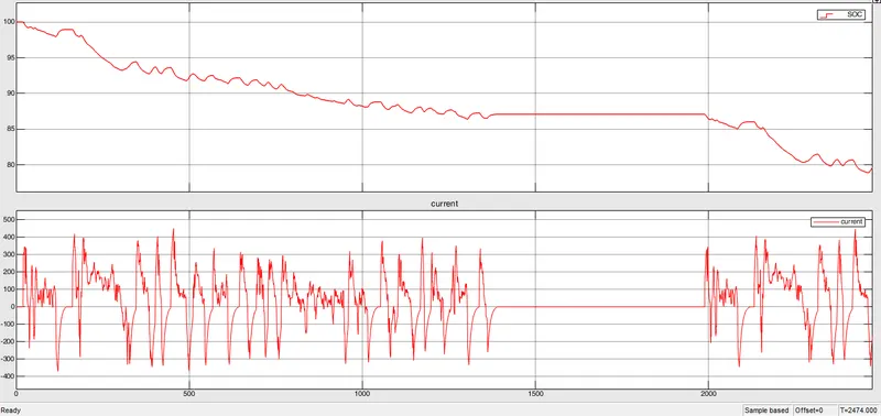
The above graph shows that remaining charge in the battery in terms of percentage after covering 17.76km of distance.

Controller Temperature:

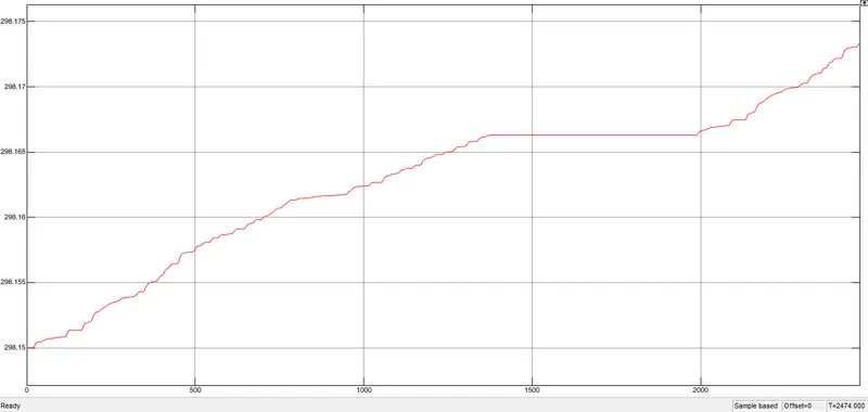
As we already know as vehicle starts to running then temperature also increases in motor controller division.

Motor Temperature:

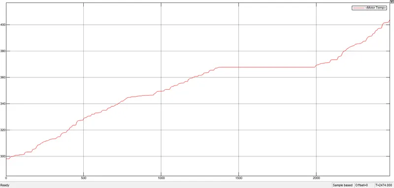
This scope result shows temperature of motor, if we again modified the pid gain values then motor temperature goes slightly reduces.

(iii) Using WOT drive cycle:

As we run the model on the FTP75 input and get them all results for tuned PID gain values. but now we were being run the model for input wide open throttle (WOT) and check how our model behaves and get the result for WOT input with tuned PID gain value and desirable other parameters.

wide-open throttle (WOT), also called full throttle, is the fully opened state of throttle on an engine (internal combustion engine or steam engine). In an Electric vehicle, WOT condition refers to the initial acceleration or time taken by the vehicle to reach maximum velocity. The maximum velocity in WOT conditions can be obtained by the electric motor characteristics of an electric vehicle.

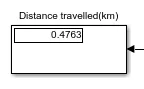
A model with WOT input and simulation time is 60sec

Input speed vs Vehicle speed:

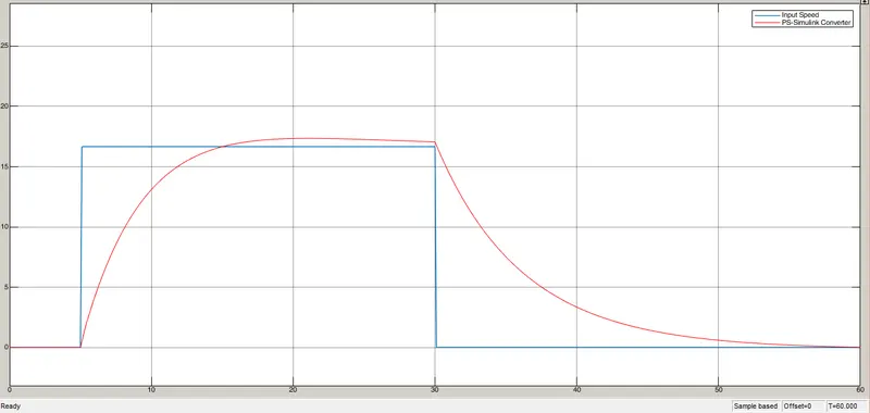
In WOT drive cycle also both input speed and vehicle speed are overlapped and they are following each other. 

Battery SOC and Current:

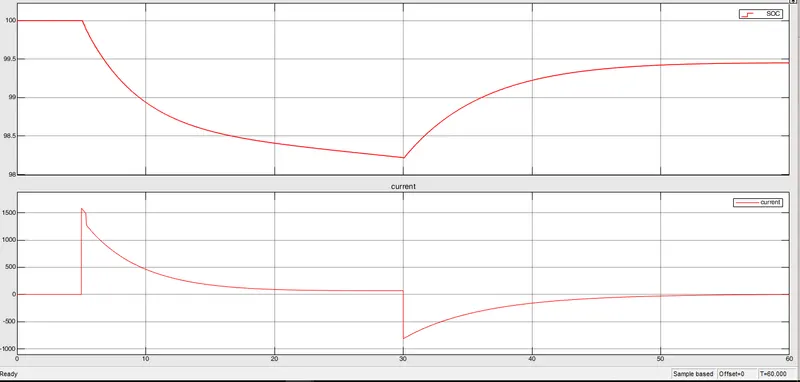
In WOT drive cycle after 60sec the battery capacity was still 99.4%

Controller Temperature:

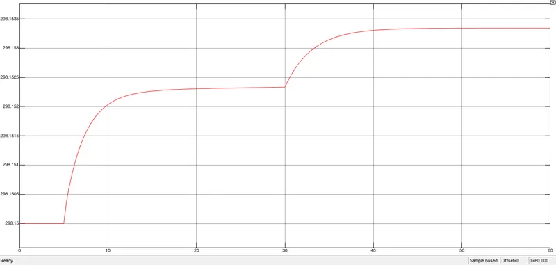
As we already know as vehicle starts to running then temperature also increases in motor controller division. 

Motor Temperature:

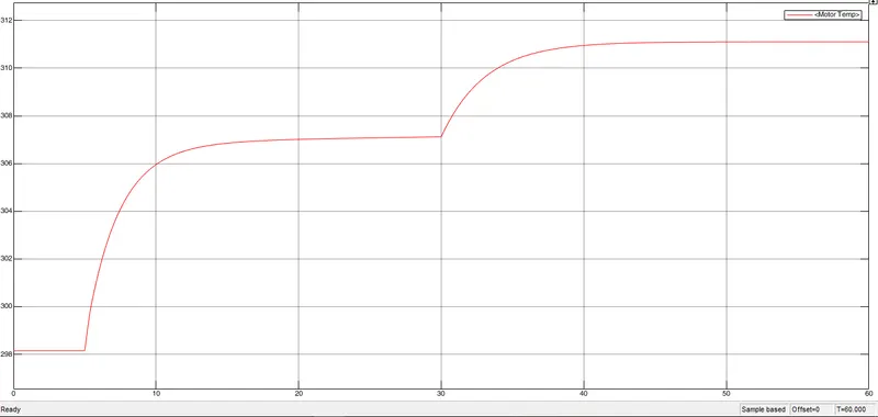
This scope result shows temperature of motor, if we again modified the pid gain values then motor temperature goes slightly reduces.

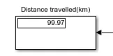
(iv) Used signal builder to reach 100km of distance: 

Input speed vs Vehicle speed:

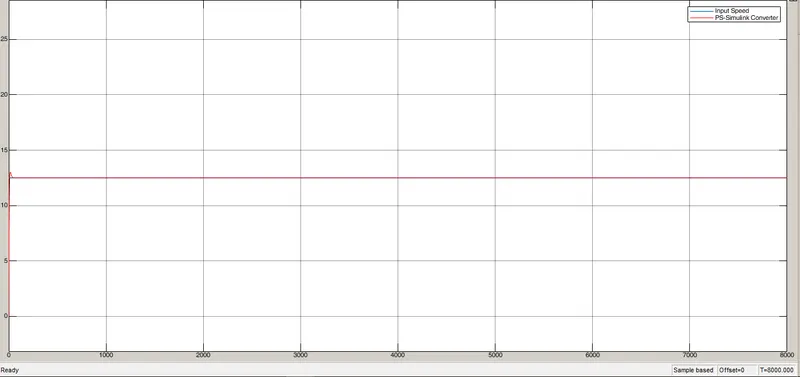
In manually prepared drive cycle also both input speed and vehicle speed are overlapped and they are following each other.

Battery SOC and Current:

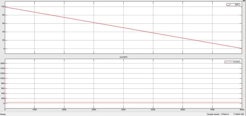
The above graph shows that remaining charge in the battery in terms of percentage after covering 99.9km of distance.

Controller Temperature:

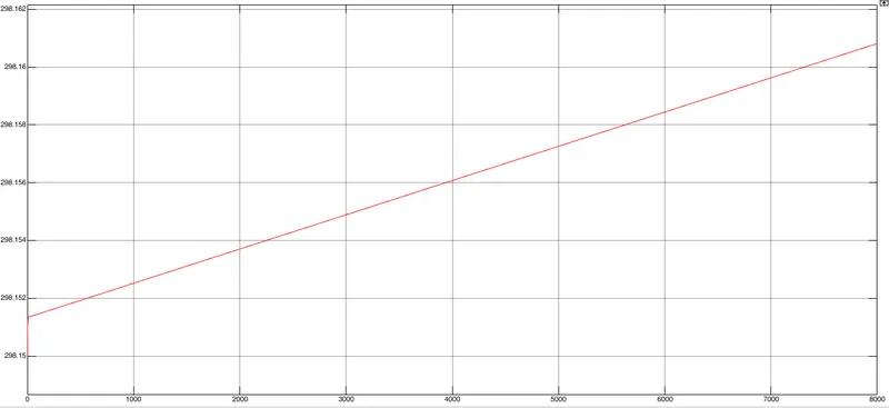
As we already know as vehicle starts to running then temperature also increases in motor controller division.

Motor Temperature:

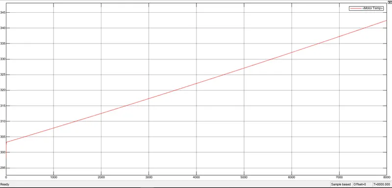
This scope result shows temperature of motor, if we again modified the pid gain values then motor temperature goes slightly reduces.

Conclusion:

From all the above cases, we understand that whatever be the input we have to set proper PID gain values for proper OUTPUT and also adjust the parameters of motor load, battery capacity is also important.

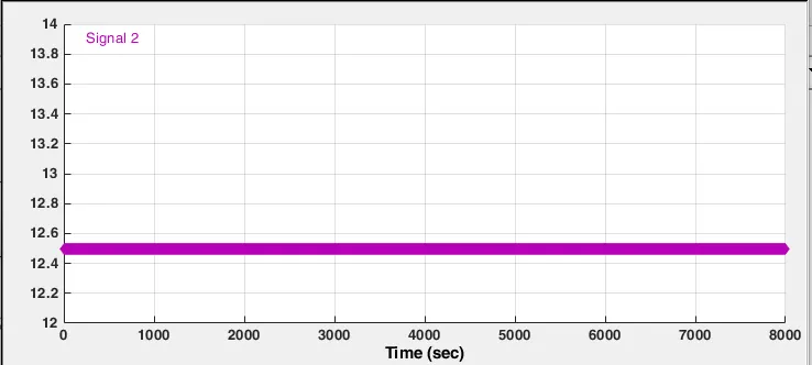
• The designed Electric Rickshaw model for the FTP75 drive cycle travels for a distance of 17.76 Km for the simulation time of 2474 secs and for WOT drive cycle travelled 0.47 Km for time of 60sec, and for constant 12.5 mph speed upto 8000sec the distance was 99.97 Km.
• And vehicle speed follows the 99% of input speed.  
• The Controller temperature for FTP75,WOT and manually prepared drive cycle was 298K,298.15K and 298.17K respectively.
• The Motor temperature for FTP75,WOT and manually prepared drive cycle was 400K,311K and 342K respectively.

-------------------------------x---------------------------------------------x------------------------------------