Free Falling Body using HYPERWORKS

AIM: To simulate and plot a free-falling body (point mass) of mass 1 kg and inertial properties 1 kgm2 in the Y-axis (gravity should be 9.81 m/s2 in the negative Y-direction, use dimension of length in meters not mm)

A screenshot of the entire interface must be attached including the plot for all the simulated cases.

Time of simulation = 2 sec

GOVERNING EQUATION: The equation to calculate the height of an object in free fall is as follows: `h = 1/2 . g. t^2` where; g = Acceleration due to gravity (m/s2) t = time (sec) THEORY: In Newtonian physics, free fall is any motion of a body where gravity is the only force acting upon it. In the context of general relativity, where gravitation is reduced to a space-time curvature, a body in free fall has no force acting on it. An object in the technical sense of the term "free fall" may not necessarily be falling down in the usual sense of the term. An object moving upwards might not normally be considered to be falling, but if it is subject to only the force of gravity, it is said to be in free fall.

SOLUTION:

Software: HyperWorks Desktop

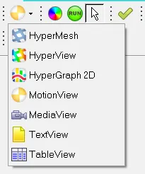
STEP 1: Select MotionView from the list of the dialogue box.

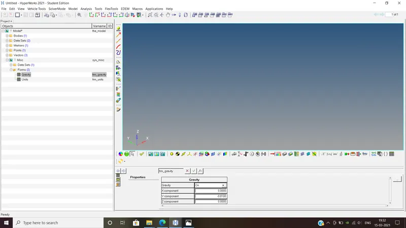
STEP 2: Check whether the gravity effect is enabled and set it to -9.81 m/s2 (negative Y-direction).

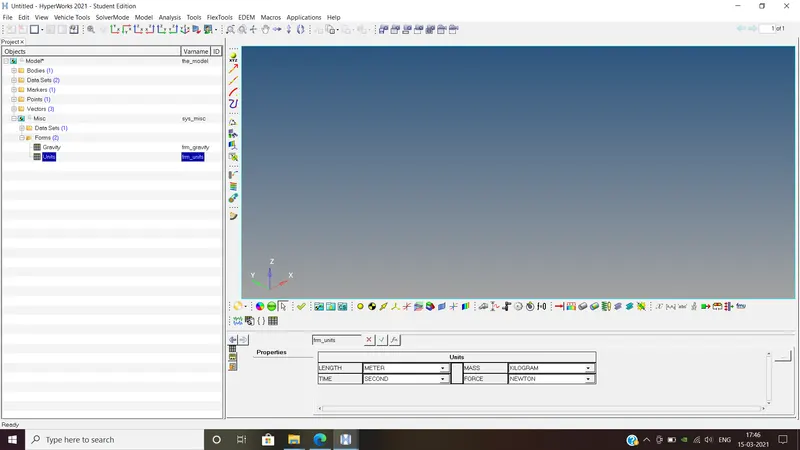
STEP 3: Set up the units for simulation from millimeter to meter as directed in the question.

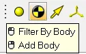
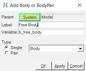
STEP 4: Select the Add Body option as shown and rename it as Free Body for reference.

The Free Body is created in the graphic window as shown below.

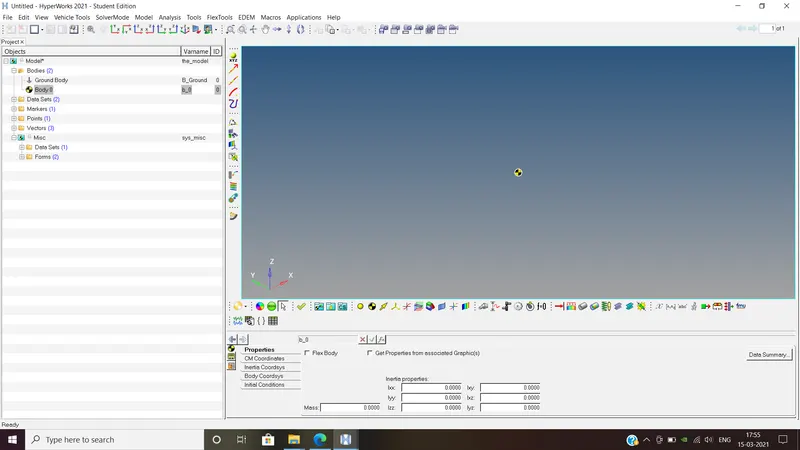
STEP 5: Assign the mass and inertia values (diagonal matrix values are sufficient i.e. `I_(x x)`, `I_(yy)` and `I_(zz)`= 1 kg.m²) as directed in the question.

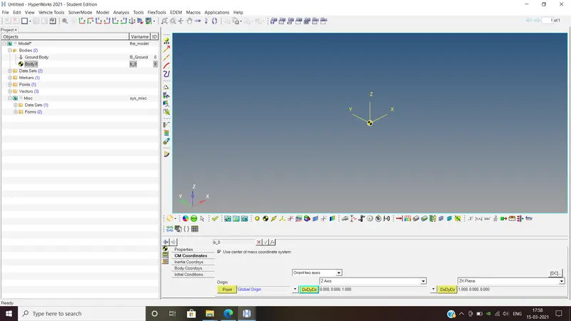
STEP 6: Check Use center of mass coordinate system and select origin point from unresolved to global origin.

The center of mass is shifted to the global origin in the graphic window as shown below.

STEP 7: Go to the Run Solver panel, set the simulation time as 2 sec. Save the model and then click Run.

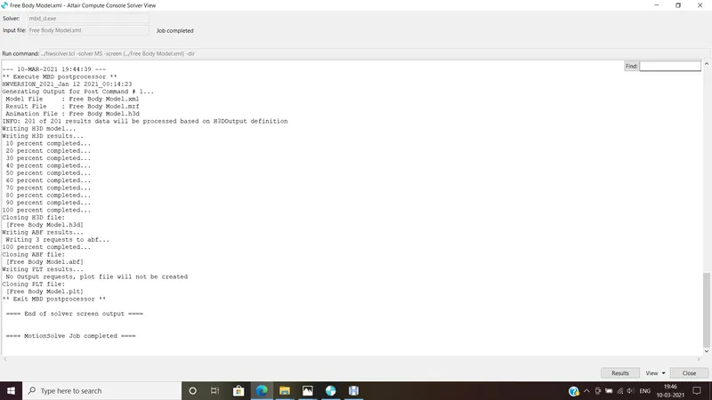
STEP 8: The processor MotionSolve runs in the background as follows.

STEP 9: Click the Plot button and select appropriate parameters to visualize the graph.

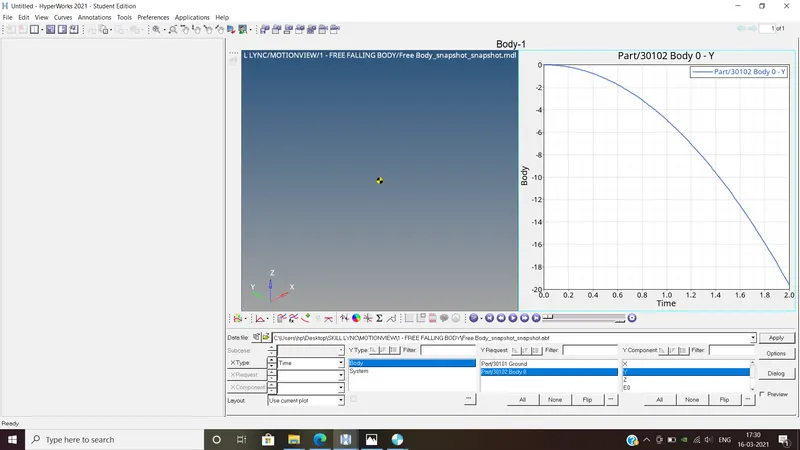
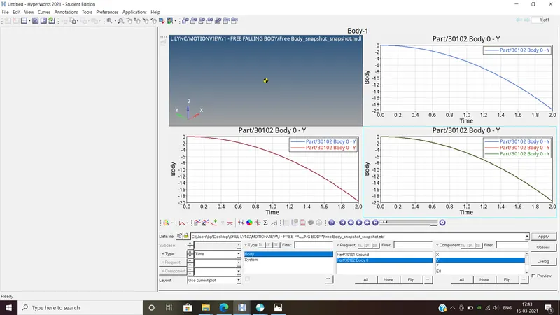
Output: The results are simulated using postprocessors HyperView (top right) and HyperGraph 2D (bottom right) as shown below.

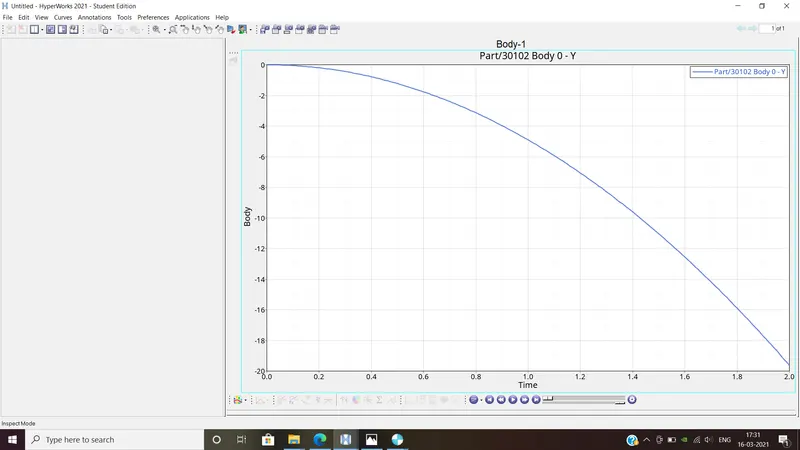
Plot: The body is falling in a parabolic fashion with respect to time (`h prop t^2`) as shown below.

Do the mass and inertial properties of the body depend on the rate of fall? Justify your answer with analytical (with equation) and simulation results.

- No, the rate of fall of a free body is irrespective of its mass and inertial properties. Any body suspended in free space will fall at the same acceleration rate (i.e. gravity).

According to Newton's 2nd Law,
`F = ma = mg`

To prove it, the properties of the free body are changed and we can see no difference in the simulation results.

m = 1 kg and I = 1 kg.m² ... (Top Right)

m = 10 kg and I = 5 kg.m² ... (Bottom Left)

m = 50 kg and I = 30 kg.m² ... (Bottom Right)

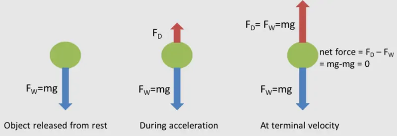
In what case will the mass have an effect on the rate of fall? In the same case what other physical characteristics will affect the rate of fall? - Yes, characteristics such as drag or air resistance and buoyant force might affect the rate of fall if considered. Drag force is given by: `F_d = 1/2 . rho . A . v^2 . C_d` Bouyant force is given by: `F_b = rho . g . v` Weight of body is given by: `W = m.g` Acceleration is given by: `a = F_(n et) / m = (W - F_d - F_b) / m` where; `rho` = Density (kg/m3) `A` = Area (m2) `v` = Velocity (m/sec) `C_d` = Drag coefficient (unitless) `m` = Mass (kg) `g` = Acceleration due to gravity (m/s2)

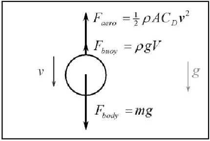When drag decreases, the rate of fall increases and vice versa. Other physical characteristics to be considered are:

- Area

- Density (Material of the object)

- Drag coefficient

- Velocity of fall

CONCLUSION: Thus, the free-falling body was simulated in HyperWorks.