Compound Pendulum using HYPERWORKS

AIM: To simulate the motion of a compound pendulum under the influence of gravity as per the figure shown below.

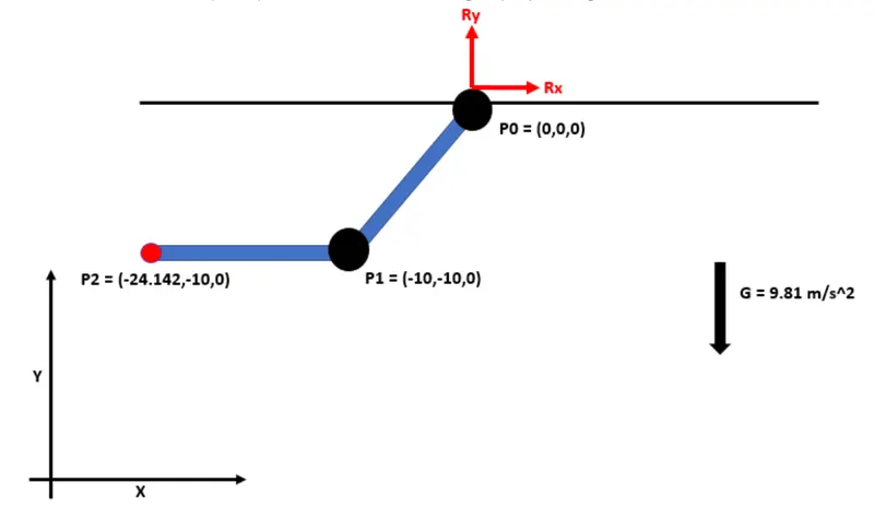
- Location of the points are shown in the figure, at P0 and P1 the rods are connected by revolute joints, all characteristic data for the rods/cylinders should be taken from the associated geometries (diameter of rods = 2m)

- You are required to plot the trace of point P2 (trace is the Y vs X displacement plot of P2 w.r.t the ground)

- Find the X and Y component of reaction forces on joint P0 vs time (Rx & Ry)

- Time of simulation = 100 sec

- Also, explain how you set up the simulation and explain the results

- Unit of length should be meters

A screenshot of the entire interface must be attached with the plot for all the simulated cases.

SOLUTION:

Software: HyperWorks Desktop

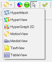
STEP 1: Select MotionView from the list of the dialogue box.

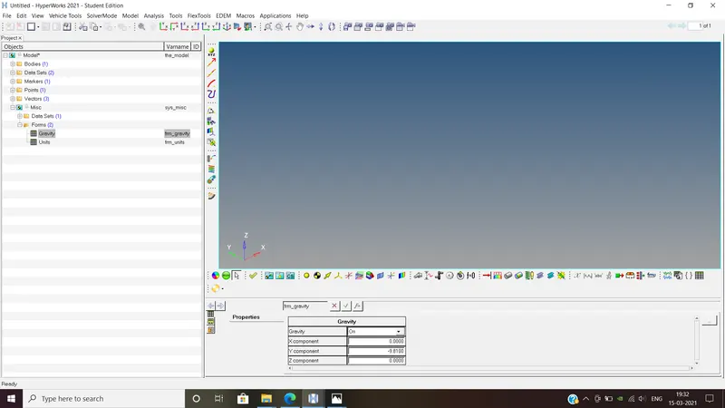
STEP 2: Check whether the gravity effect is enabled and set it to -9.81 m/s2 (negative Y-direction).

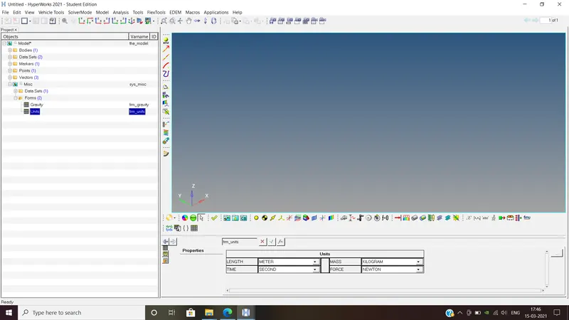
STEP 3: Set up the units for simulation from millimeter to meter as directed in the question.

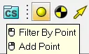
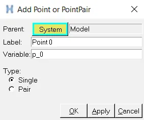
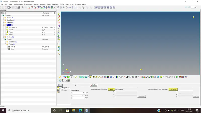
STEP 4: Select the Add Point option as shown and create Point 0 (0,0,0), Point 1(-10,-10,0) and Point 2 (-24.142,-10,0).

The points are created in the graphic window as shown below. (Click on the screen and press F to fit the screen)

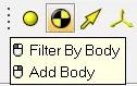
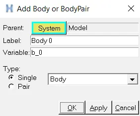
STEP 5: Select the Add Body option as shown and create Body 0 and Body 1. Also tick the Get Properties from associated Graphic(s) to obtain meaningful mass and inertia values.

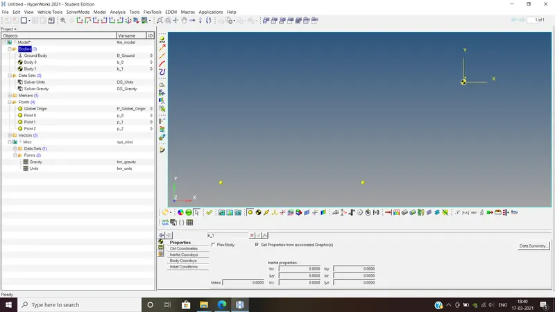
The bodies are created in the graphic window as shown below.

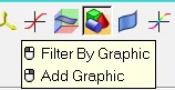
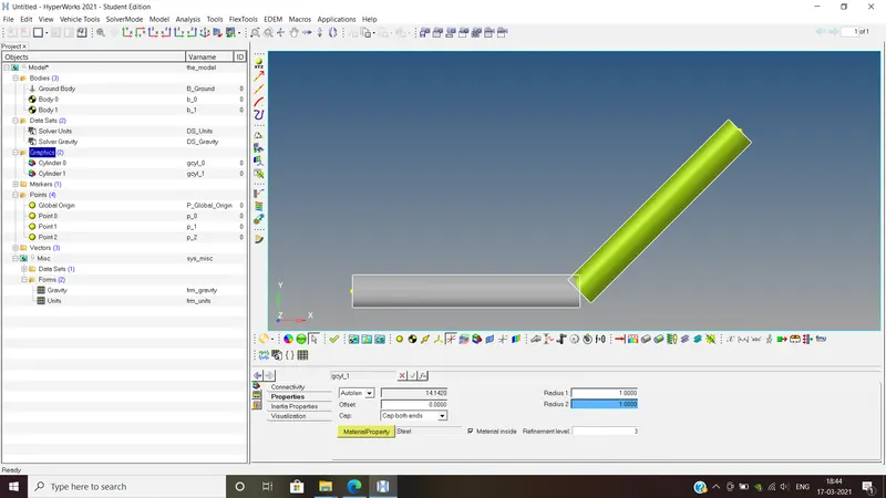
STEP 6: Select the Add Graphics option and add Cylinder 0 and Cylinder 1.

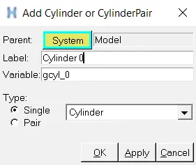
From Connectivity, Cylinder 0 was given Body 0 as parent body with origin as Point 0 and direction as Point 1.

Cylinder 1 was given Body 1 as parent body with origin as Point 1 and direction as Point 2.

From Properties, the radius of the cylinder was set to 1m (since diameter = 2m).

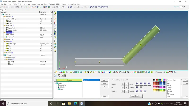
STEP 7: Select the Graphic Entity Attributes option and tick Opaque - Transparent for better visibility.

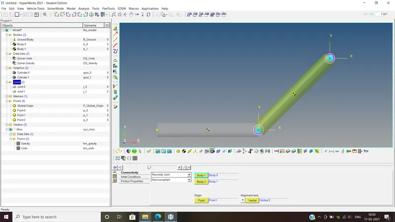
STEP 8: Select the Add Joint option and add Joint 0 and Joint 1.

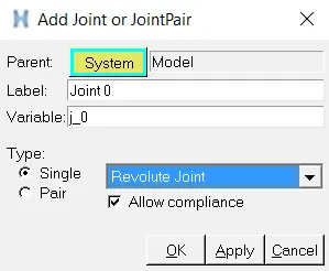
Joint 0 was given Body 1 as Ground Body and Body 2 as Body 0 with origin being Point 0 and alignment axis vector as Global Z.

Joint 1 was given Body 1 as Body 1 and Body 2 as Body 2 with origin being Point 1 and alignment axis vector as Global Z.

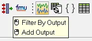
STEP 9: Select the Add Output option and add Output 0 and Output 1.

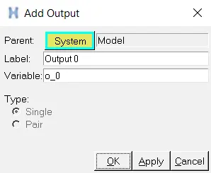
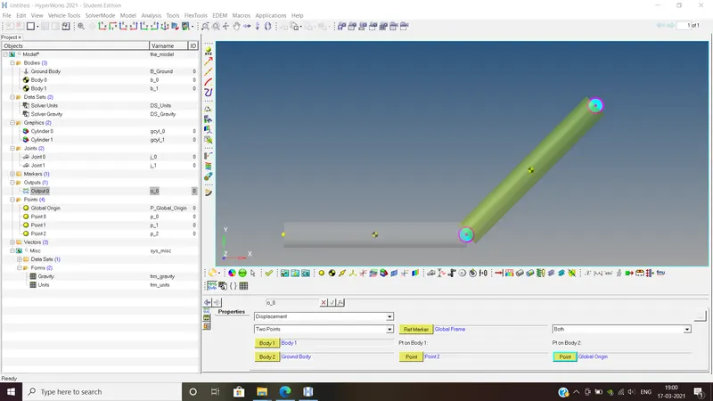
Output 0 was selected as Displacement and given Body 1 as Body 1 and Body 2 as Ground Body with point on Body 1 being Point 2 and point on Body 2 being Global Origin. (as trace of point 2 was to be plotted)

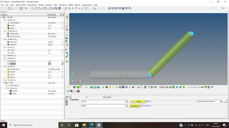
Output 1 was selected as Force and measurement given to Entity and assigned to Body 0.

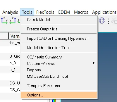
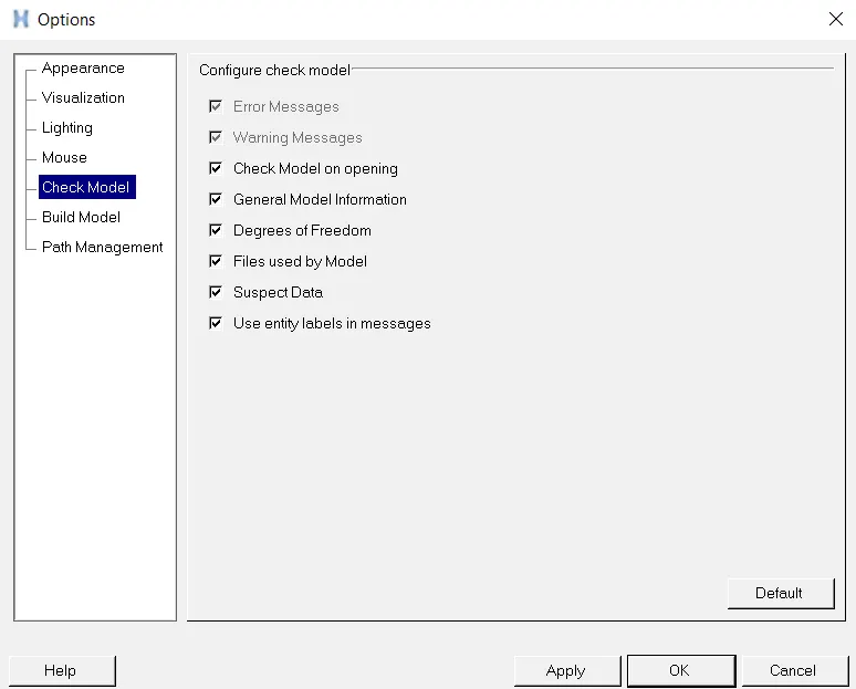
STEP 10: Select Tools - Options - Check Model and tick all the boxes as shown below.

Again go to Tools - Check Model - DOF to check the details of our model.

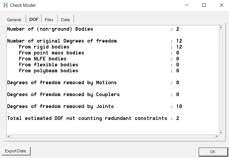
STEP 11: Go to the Run Solver option, set the simulation time as 100 sec. Save the model and then click Run.

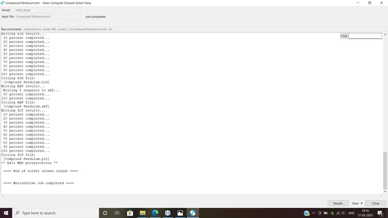
STEP 12: The processor MotionSolve runs in the background as follows.

STEP 13: Click the Plot and Animate button and select appropriate parameters to visualize the graphs and simulation.

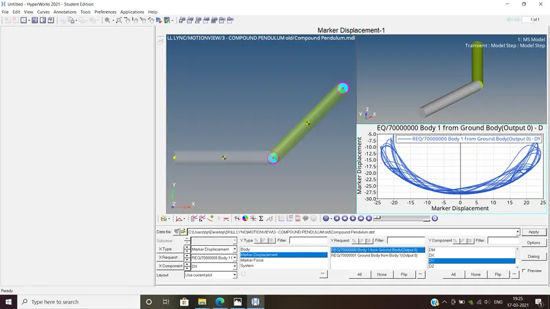
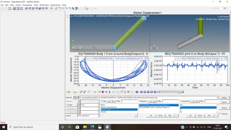
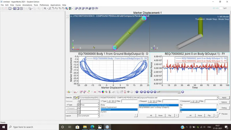
Output: The results are simulated using postprocessors HyperView (top right) and HyperGraph 2D (bottom) as shown below.

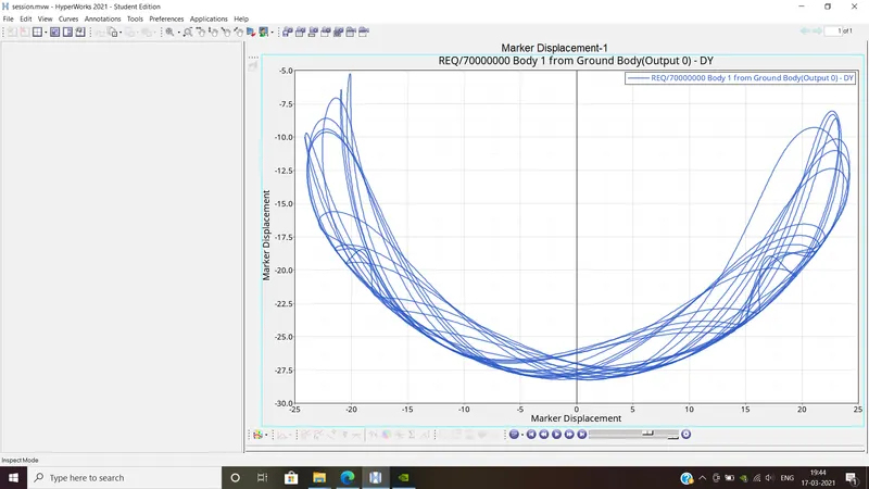
Plot #1: The plot for Y displacement vs X displacement of Point 2 (i.e. trace of Point 2) with respect to the ground is shown below.

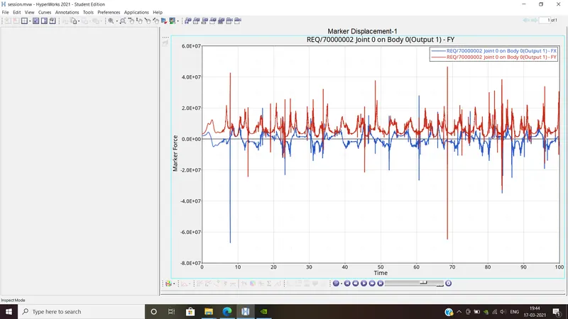
Plot #2: The plot for X component and Y component of reaction forces on joint P0 vs time (Fx & Fy) is shown below.

CONCLUSION: Thus, the compound pendulum was simulated in HyperWorks.