External Flow Simulation Over a Cylinder in SolidWorks

Aim: To do the transient flow simulation over the cylinder in SolidWorks.

Objective:

• The main objective of this project is to peform the Flow Simulation over a cylinder in SolidWorks.
• To obtain the value of Reynold's number using the given inlet velocity of fluid = 10 m/s
• With the obtained value of Reynold's number from above case, the Reynold's number has to be increase by a factor of 20%, 40%, and 100% and find the inlet velocity of fluid.
• To run the transient flow simulation for all the above cases.

Cases	Reynold's number value	Inlet velocity
Case 1	To be found	10 m/s
Case 2	Re to be increased by 20% obtained from Case 1	To be found
Case 3	Re to be increased by 40% obtained from Case 1	To be found
Case 4	Re to be increased by 100% obtained from Case 1	To be found

1. Introduction

:Laminar flow:

• Laminar flow occurs when the fluid flows in infinitesimal parallel layers with no disruption between them.
• In Laminar flows, fluid layers slide in parallel with no eddies, swirls or currents normal to the flow itself.

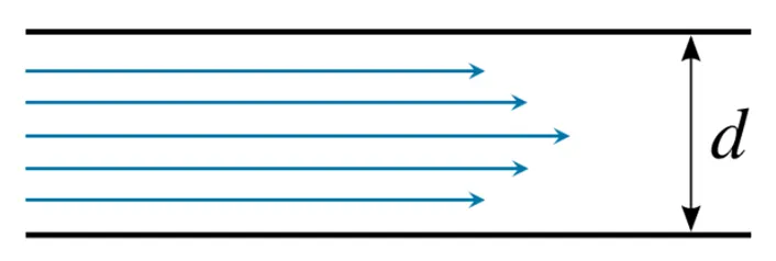
Fig. Laminar flow in closed pipe

Turbulent flow:

• In fluid dynamics, a turbulent means irregular flows in which eddies, swirls, and other flow instabilities occur.
• Turbulence is commonly observed in everyday phenomena such as fast flowing rivers, smoke from chimney, etc.

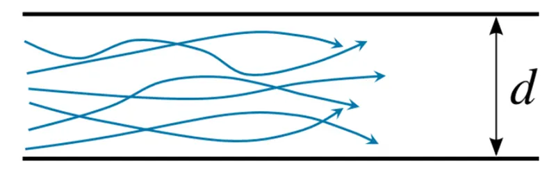
Fig. Turbulent flow in closed pipe

Reynold’s number:

• The Reynold’s number (Re) is a dimensionless number expressing the ratio between inertial force and viscous force.
• The Reynold’s number is a mathematically defined as:

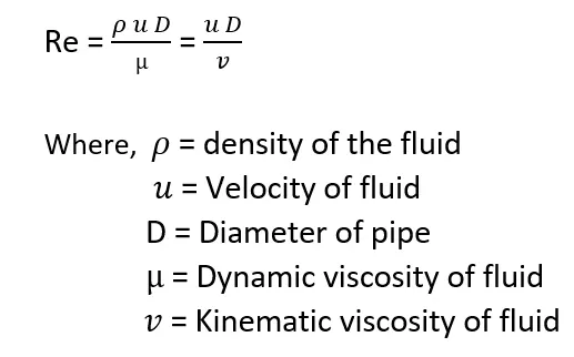
• At low values of Re, the flow is Laminar. But when Re exceeds a certain threshold, semi-developed turbulence occurs in the flow, this regime is referred to as Transition regime and occurs for a certain range of the Reynold’s number.
• Finally, over a certain value of Re, the flow becomes fully

Viscosity:

• The resistance of a fluid to flow when subjected to a force is called Viscosity.

Dynamic Viscosity

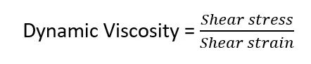
• The unit of measurement of Dynamic Viscosity is Pa s or N s/m²
• Dynamic Viscosity is also known as Absolute viscosity.

Kinematic Viscosity

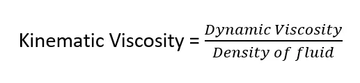
• The unit of measurement of Kinematic Viscosity is m²/s
• Kinematic Viscosity is also known as Diffusivity of Momentum.

________________________________________________________________________________________________________

2. Calculations:

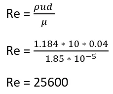
Case:1 (Baseline case of Simulation)

With the help of formula,

and u = 10 m/s

Case : 2

Increasing the Reynold's no of case 1 by a factor of 20%, we get

Re = 30720 and Flowspeed u = 12 m/s

Case : 3

Increasing the Reynold's no of case 1 by a factor of 40%, we get

Re = 35840 and Flow speed u = 14 m/s

Case : 4

Increasing the Reynold's no of case 1 by a factor of 100%, we get

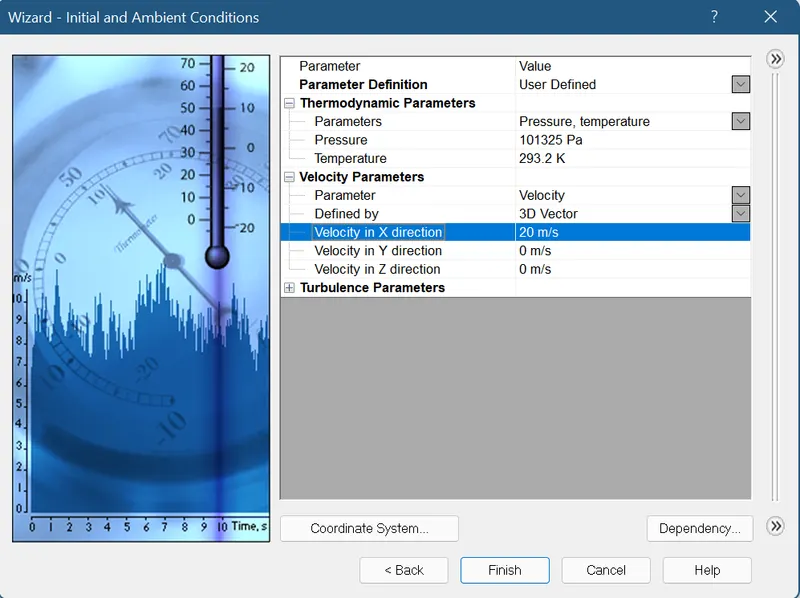
Re =51200 and Flow speed u = 20 m/s

Cases	Reynold's number	Flow Speed
Case 1	25600	10 m/s
Case 2	30720	12 m/s
Case 3	35840	14 m/s
Case 4	51200	20 m/s

___________________________________________________________________________________________________

Calculation of simulation time:

Domain length= 0.5m

We know that,

Time = Distance/speed

Therefore, Time = 0.5/10

= 0.05 Seconds

Now the Simulation time should be twice

Therefore, Simulation time = 0.1 Seconds

_____________________________________________________________________________________________

3. Model Preparation of Cylinder

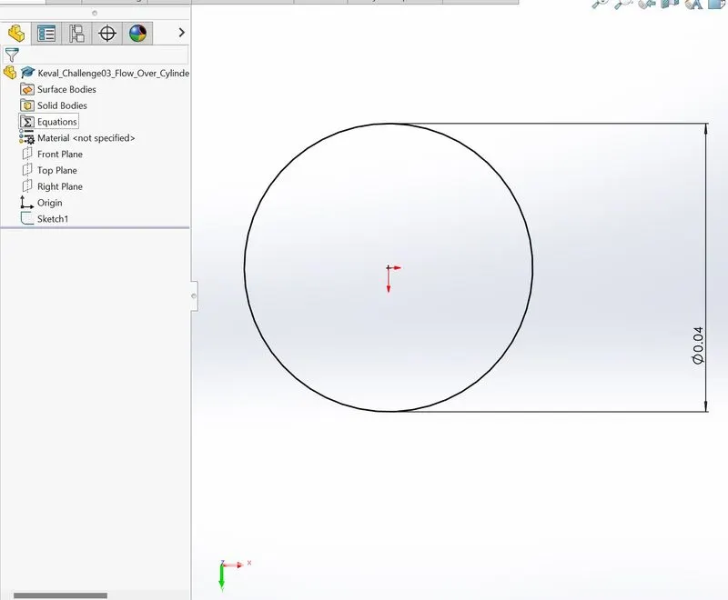
1. Preparation of sketch

Circle of diameter 0.04m was created

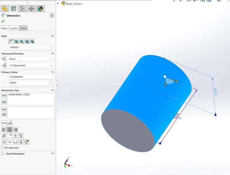
2. Extrude Boss/Base

Length = 0.05m

_____________________________________________________________________________________________________

4. Flow simulation:

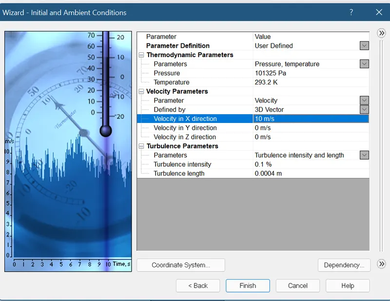
Case 1 : Inlet flow velocity(u) = 10m/s in X-Direction

Step:1

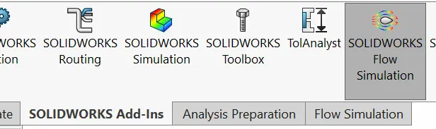
Step:2

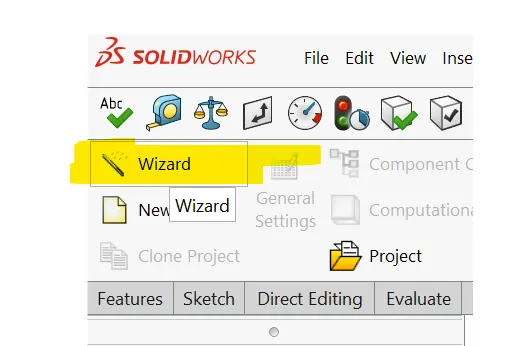
Step:3

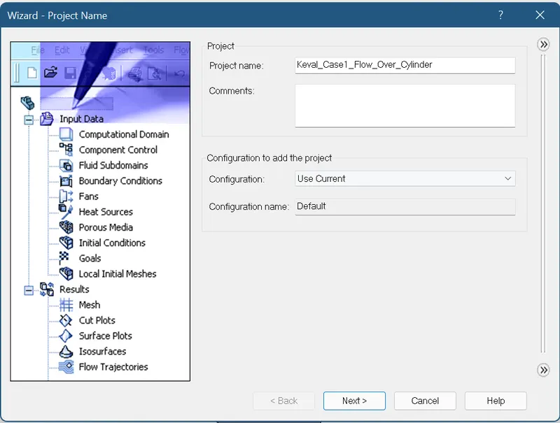
Step:4

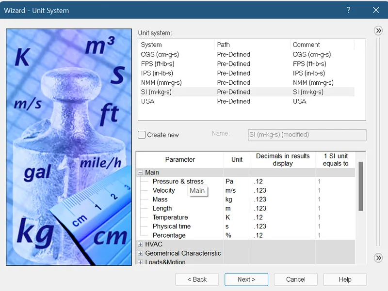
Step:5

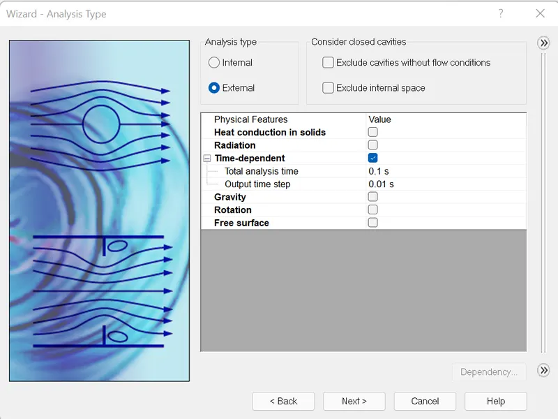
Step:6

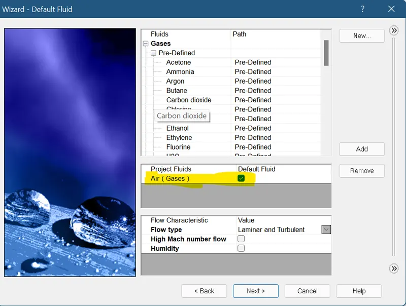
Step:7

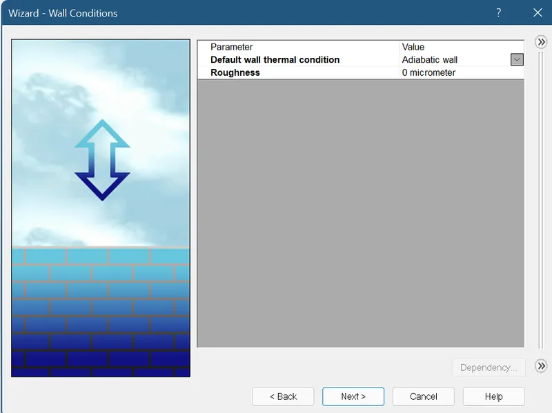
Step: 8

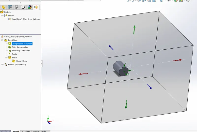
After finishing, we get the bounding box around the cylinder is created

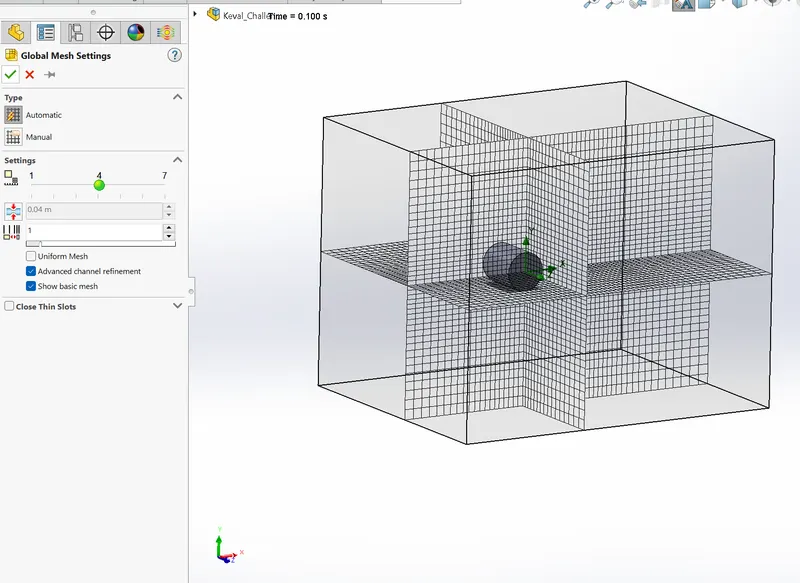
Meshing:

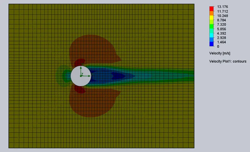
Results of Case:1

Velocity Plot of Case:1

Animation of velocity plot Case 1:

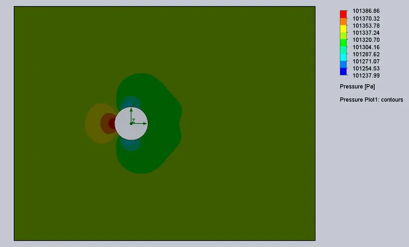
Pressure Plot of Case 1:

Animation of pressure plot Case1:

____________________________________________________________________________________________

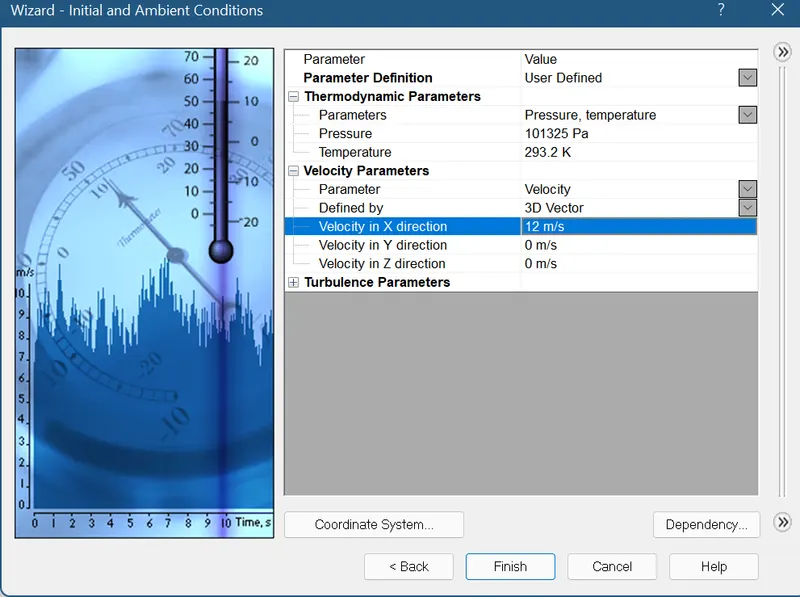
Case 2: Inlet Flow velocity =12 m/s in X-direction:

Step-1 to Step-7 are same as of Case : 1 (i.e. u=10m/s)

Now, Step-8

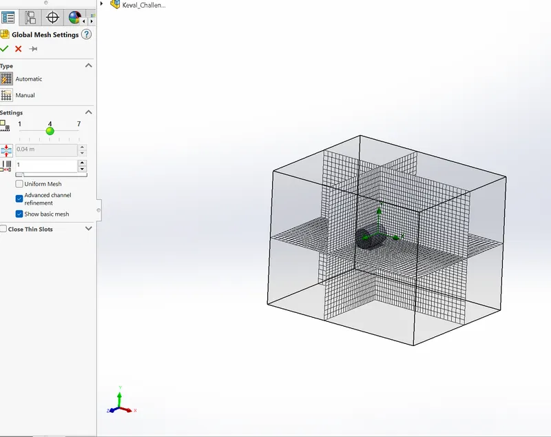
Meshing:

Results of Case 2:

Velocity plot of Case 2:

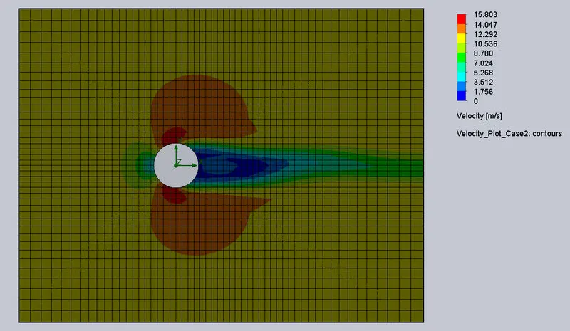
Animation of Velocity Plot of Case 2:

Pressure plot of Case 2:

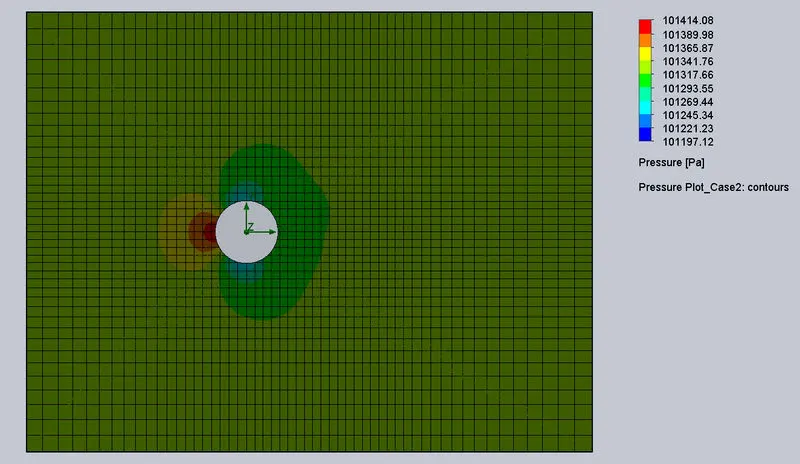
Animation of pressure plot of Case-2

Case:3 Inlet Flow velocity = 14m/s in X-direction

Results:

Velocity plot of Case-3

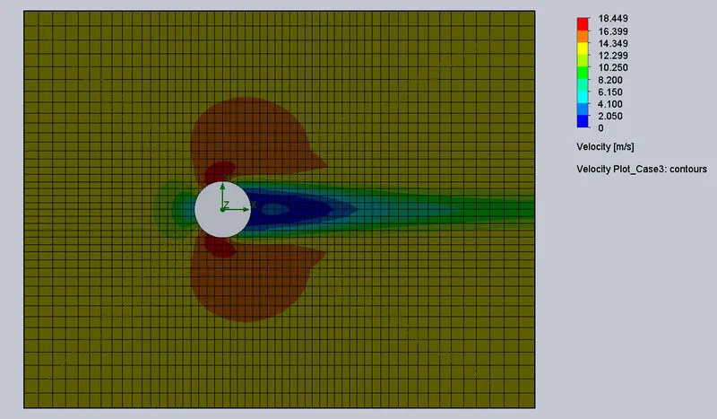
Animation of Velocity plot of Case-3

Pressure plot of Case:3

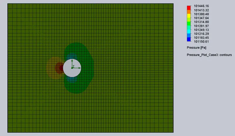
Animation of pressure plot of Case-3

Case : 4 Inlet flow velocity = 20 m/s in X-direction:

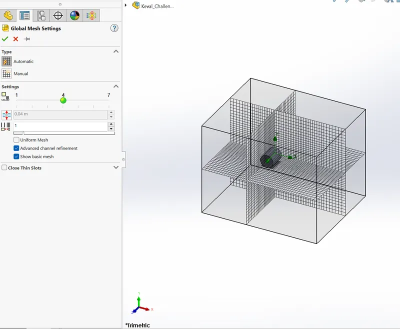
Meshing:

Results:

Velocity plot of Case;4

Animation of Velocity plot of Case-4

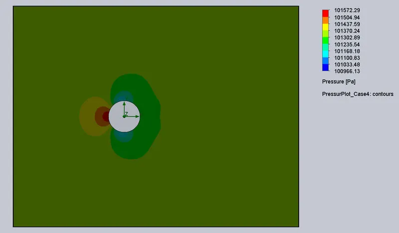
Pressure plot of Case-4

Animation of pressure plot of Case-4

Observation Table:

Cases	Reynold's Number	Initial Velocity	Maximum Velocity (m/s)	MinimumVelocity (m/s)	Maximum Pressure (Pa)	Minimum Pressure (Pa)
Case-1	25600	10 m/s	13.176	0	101386.66	101237.99
Case-2	30720	12 m/s	15.803	0	101414.08	101197.12
Case-3	35840	14 m/s	18.449	0	101446.16	101150.61
Case-4	51200	20 m/s	26.457	0	101572.29	100966.13

From the above table and plots we can clearly see that:

• As the Reynold's number is increased the velocity increases.
• From plots and animation we can see that the maximum pressure occurs at the starting point where the air flow strikes the wall of the cylinder and hence the velocity will be minimum.
• When the flow of air strikes the cylinder the velocity of air gets dispersed over the cylinder.
• From plots we can see the red region indicates the maximum velocity whih in all the cases occurs at the initial phase, while the dark blue region indicates the minimum velocity which is in the front section of the cylinder as the air flow is being resisted by the cylinder.

Conclusion:

From this project we can conclude that the SolidWorks Flow Simulation helps to quickly simulate air flow around the designs (cylinder) and helps to improve the design.