DC-DC Converter
1a) Explain the following terms and note down their mathematical formulae.
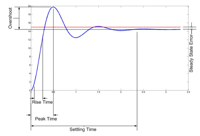
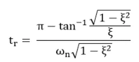
- Rise time: time it takes for the response to rise from 10% to 90% of the steady-state response
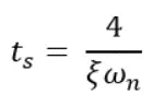
- Settling time: the time taken for the signal to be bounded to within a tolerance of 2-5% of the steady state value
- Peak overshoot: maximum overshoot is the maximum peak value of the response curve measured from input step value
(max value − final value)/final value × 100
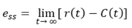
- Steady state error: the difference between the input step value (dashed line) and the final value
b) Tune a compensator for DC Motor Using Bode Diagram Graphical Tuning. The transfer function is given as:
`G=1.5/(s^2+14s+40.02)`
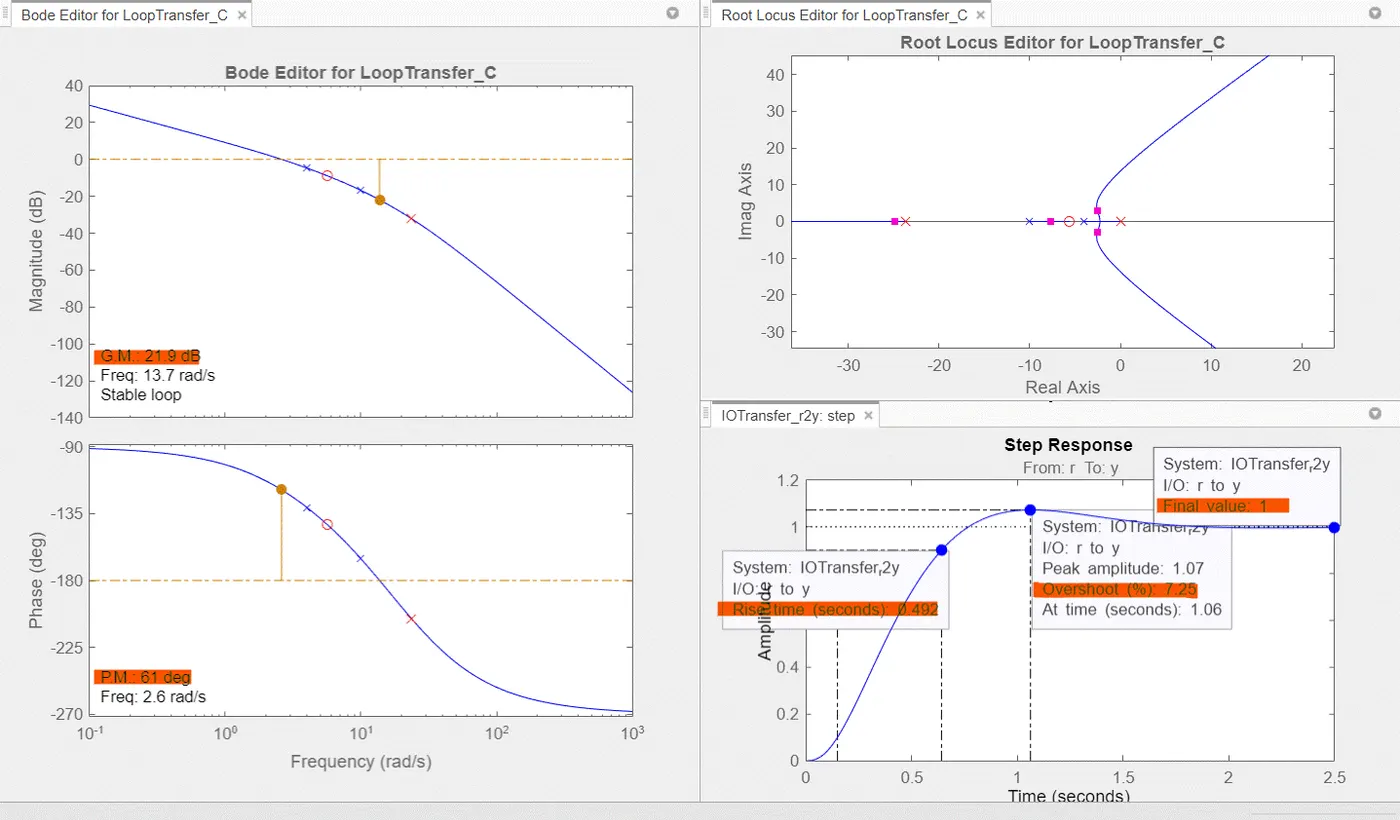
Meet the following specifications - Rise time less than 0.5 seconds, Steady-state error of less than 5%, Overshoot of less than 10%, Gain margin greater than 20 dB, Phase margin greater than 40 degrees
- To achieve rise time < 0.5sec and overshoot < 10%, the Proportional gain (Kp) is adjusted at first. Kp can be thought of as the powerful motor, powerful battery & ultracapacitor to achieve peak acceleration, top speed, and high power density related parameters. However, adjusting just the gain doesn't allow to achieve steady state error < 5% as the step response can get to a maximum of about 0.8, whereas at least 0.95 is needed to satisfy conditions. So although increasing Kp allows to reduce rise time and overshoot, it is insufficient to meet other conditions.
- This is where an Integral controller (Ki) comes in. Ki can be thought of as the optimizer which will allow the use of the power sources as effectively as possible to achieve high energy density along with high power density in order to achieve final output. Adding an integrator eliminates the steady state error and the step response converges at 1. However, at this point, while every other condition is met, the rise time goes beyond 0.5 seconds.
- This is where a lead compensator comes in. A lead compensator is a combination of a pole and zero added to the already existing poles and zeroes. Although this procedure involves trial and error for the placements of the pole and zero, the point is to make the added pole a larger negative number than the added zero to shift the entire root locus to the left, as that improves the stability and the system's response speed (i.e. rise time).
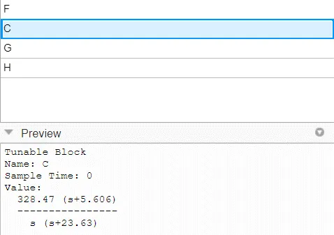
- There isn't just one combination that works here, but placing the zero at -5.6 and the pole at -23.6 was enough to meet all the requirements, as can be seen in the figure below.
- A 'Proportional-Integral' or 'PI' controller was used here along with a phase lead compensator to meet the requirements. The 'D' or 'Derivative' controller, part of 'PID', was unnecessary here since no fluctuations or vibrations needed a damping effect.
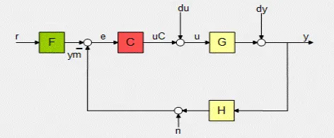
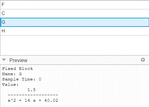
- This is typically how the closed loop feedback system for this kind of problem would look like. As is seen below, the 'C' or the 'Compensator' block has an added integrator along with a lead compensator (pole and zero) that can be fed to the plant function 'G'.
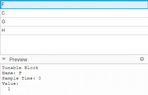
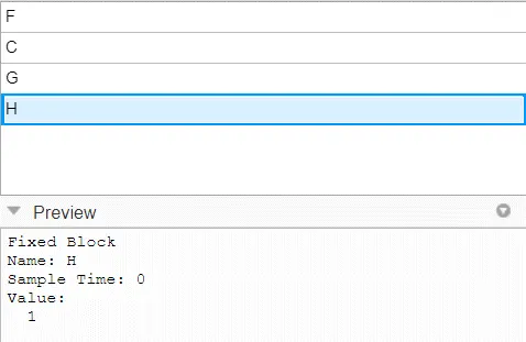
- As the steady state error was eliminated by the addition of an integrator, the value of F and H are identical as there is no difference between the input 'r' and the output 'y'
2) Can a system with a pole on the right half of the s-plane be stable? Justify your answer with an example.
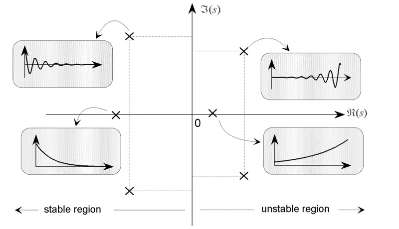
- For a Linear Time Invariant (LTI) system, if an input is bounded, the output must be bounded too
Taking an example as simple as:
`H(s)=s/((s+2)(s-1))`
The poles are s = -2 and s = 1
Laplace(H(s)) = H(t)
`H(t)=K_1*e^(-2t)+K_2*e^t`
The first term is a decaying term while the second is a rising term. This is one of the benefits of applying Laplace transformation - it allows us whether the output is bounded or not.
Since the second term is rising (refer to figure above) indefinitely, it means its output is not bounded and hence the system is unstable. For the system to be stable, both poles would have to be in the left half of the s-plane.
Another way is to use the root-locus method.
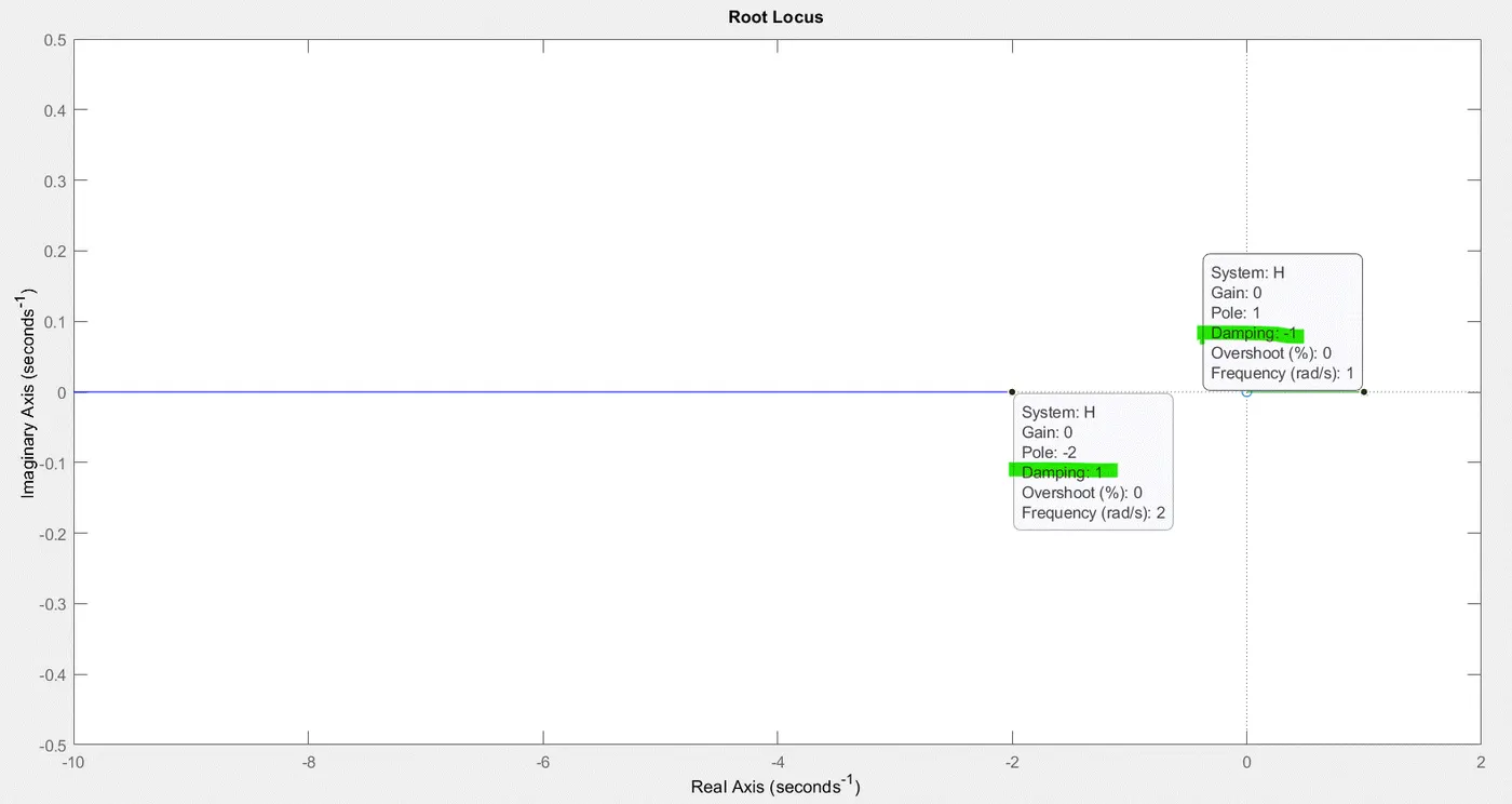
Plotting the same example: `H(s)=s/((s+2)(s-1))`
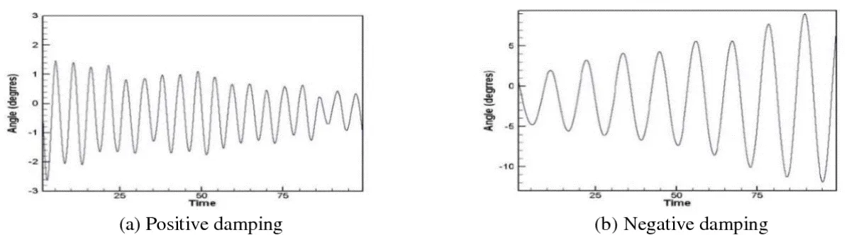
For the 2 poles i.e. s = -2 and s = 1, it shows the damping coefficient. For the pole s = 1, the damping coefficient is -1. A negative damping coefficient means continuous increase in amplitude, which means an unbounded output and thus an unstable system.
3) Use the following link of Synchronous Buck Converter in order to solve the following questions:
a) Run the simulation for the default values and comment on the results with respect to stability of the system.
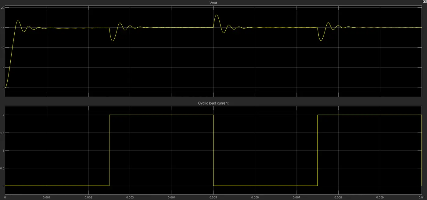
- Output voltage is bounded and stabilizes at 15V, hence the system is stable
b) Change the reference voltage and comment on whether it is tracking the reference voltage or not.
Changed reference voltage from 15V to 5V:
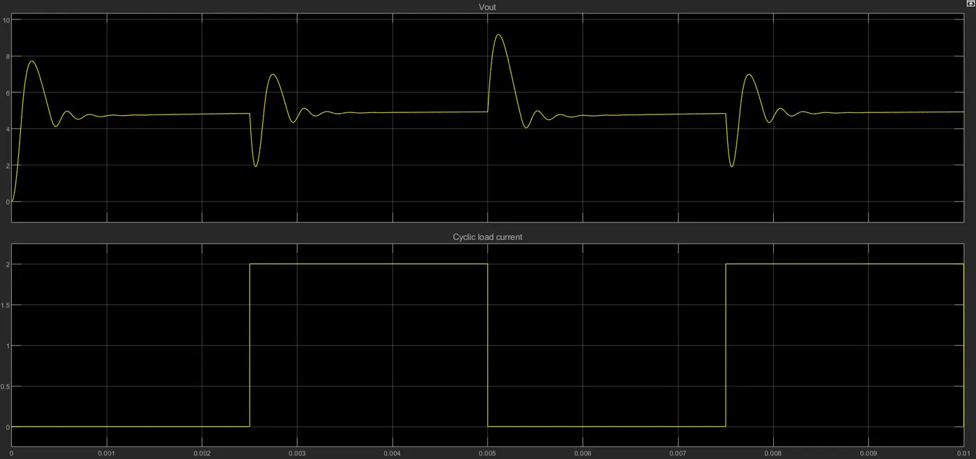
- Reference voltage is being tracked as is evident. A cyclic load has been applied which is why the output is repetitive. It constantly stabilizes at the reference voltage before repeating the entire cycle again.
Changed reference voltage from 15V to 25V:
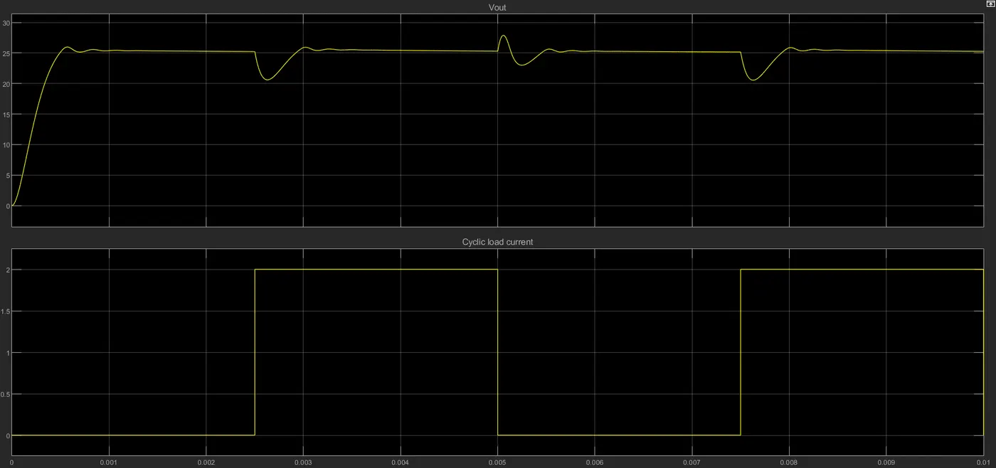
- Reference voltage is tracked here as well as the system stabilizes at 25V constantly.
- The ability of the system to track the reference voltage is seen through these changes. This is made possible due to the feedback control system and the PID controller, which constantly adjust the system to meet the requirements of the reference given.
c) Change the PI gain values and comment on the stability of the system w.r.t. new values.
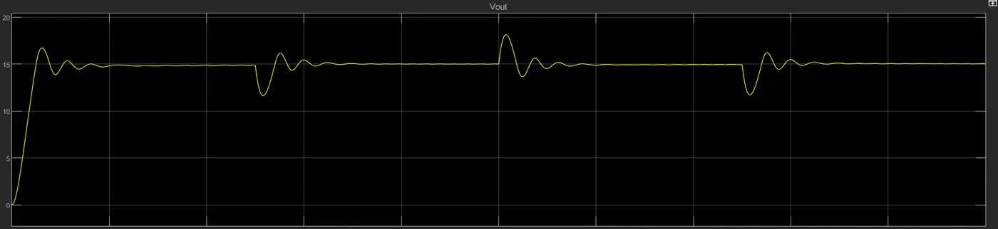
1) Kp - 0.5, Ki - 200 (DEFAULT)
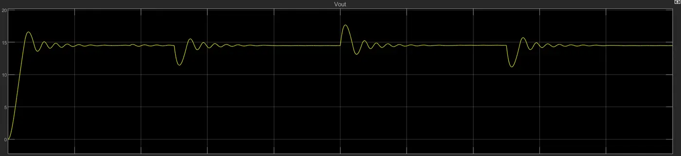
2) Kp - 1, Ki - 1
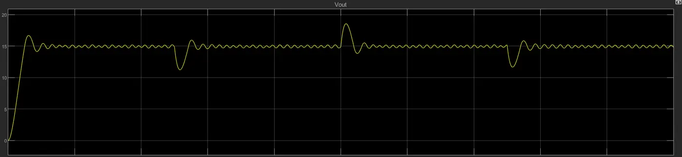
3) Kp - 10, Ki - 10
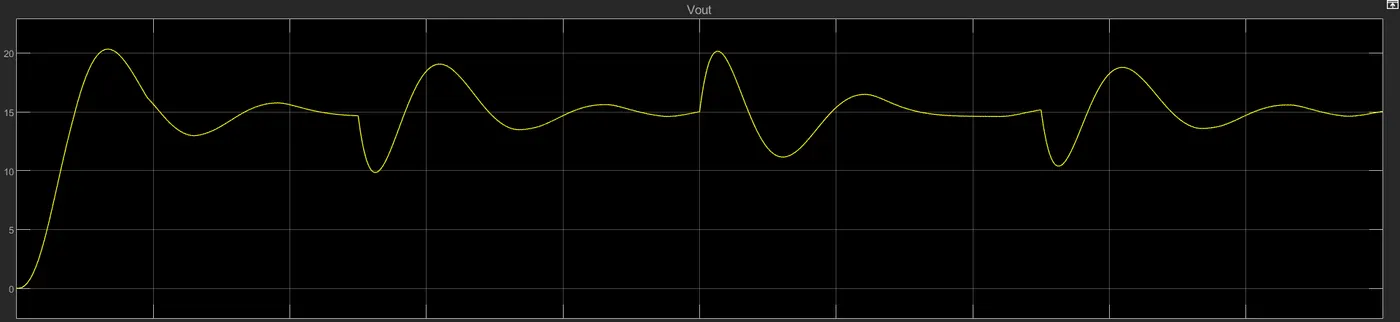
4) Kp - 0.01, Ki - 200
- It can be concluded from the above graphs that a balance between Kp and Ki is crucial. Insufficient Ki will lead to larger steady state error as is seen in Graph 2, so that is undesirable.
- If Ki is good enough but Kp is too low, that will lead to huge rise time, overshoot, and settling time with too many fluctuations and thus an unstable system.
- Graph 1 is the most stable system while Graph 4 is the least stable.
d) Change the switching frequency and comment on the stability of the system w.r.t. new values.
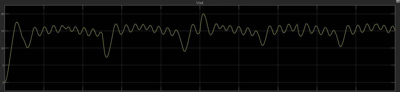
500Hz:
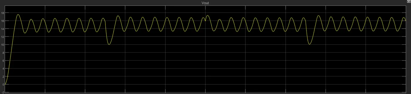
10,000Hz:
250,000Hz:
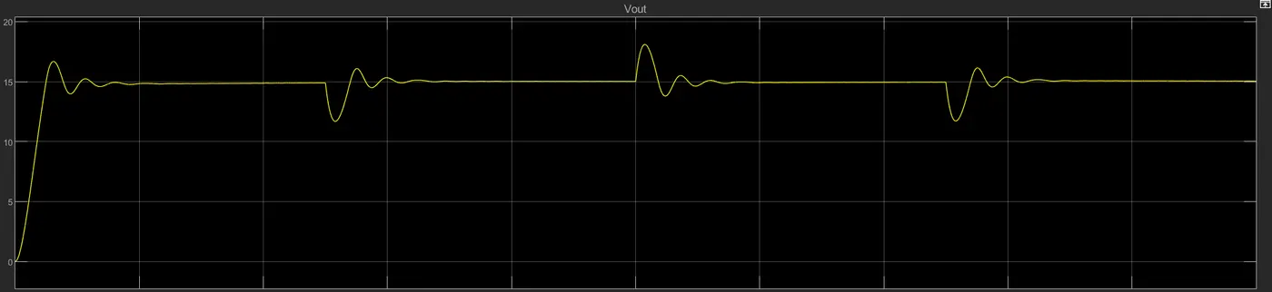
Switching frequency refers to the number of times the switch changes state (on/off) per second. As the switching frequency increases, fluctuations in the output are reduced, as is evident. Settling time is much longer with lower switching frequencies, and due to higher voltage ripples, the stability of the system is lower.
With higher switching frequency, smaller inductor and capacitor are needed as well, and a better dynamic performance can be achieved.
However, due to higher switching losses (which are the main losses in power converters), efficiency is reduced as more power is lost in the form of heat.