Ahmed Body Challenge
Ahmed Body Project:-
Run the simulation for the velocity of 25 m/sec with the default air properties in fluent.
For this challenge, you will have to provide answers to the following questions:
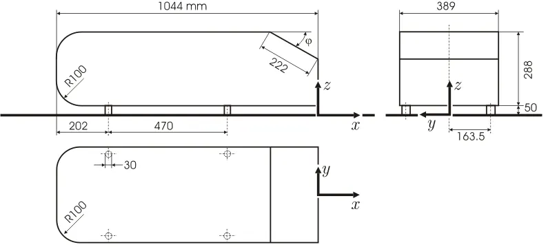
Q1. Describe Ahmed's body and its importance.
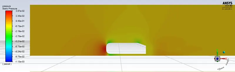
Q2. Explain the reason for the negative pressure in the wake region.
Q3. Explain the significance of the point of separation.
Expected Results:
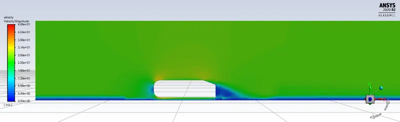
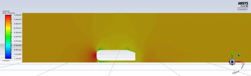
1. Velocity and pressure contours.
2. The drag coefficient plot for a refined case.
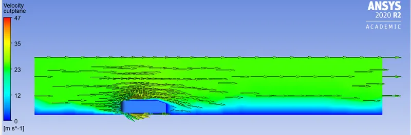
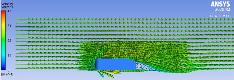
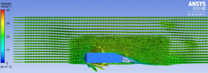
3. The vector plot clearly showing the wake region.
4. Perform the grid independency test and provide the values of drag and lift with each case.
Q1. Describe Ahmed's body and its importance.
The Ahmed Body was first created by S.R. Ahmed in his research “Some Salient Features of the Time-Averaged Ground Vehicle Wake” in 1984. Since then, it has become a benchmark for aerodynamic simulation tools. The Ahmed body is a benchmark model widely used in the automotive industry for validating simulation tools. The Ahmed body shape is simple enough to model, while maintaining car-like geometry features. The importance of Ahmed's body is to understand the flow processes involved in drag production. Through understanding the mechanisms involved in generating drag we can design a car to minimize drag and minimize fuel consumption and maximize performance.
Q2. Explain the reason for the negative pressure in the wake region.
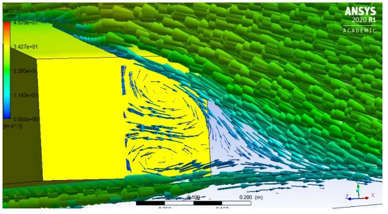
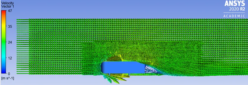
when velocity flow is higher, there should be low pressure. And in ahmed body simulation case, the pressure is high enough to detach layer from the body while velocity and shear stress become zero and create a wake region. There is a negative velocity gradient and shear stress due to the flow circulation which causes reversible highly turbulent flow as shown in velocity vector contour. But fluid has to move against the adverse pressure gradient resultant there should be low pressure inside the wake reason which responsible for drag force.
Q3. Explain the significance of the point of separation.
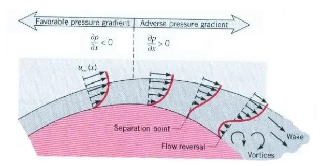
The point of separation in turbulent flow is the detachment of a boundary layer from a surface into a wake in an external flow problem. Due to the friction forces, velocity starts decreasing and also gets an increase in pressure. Flowing against an increasing pressure is known as flowing in an adverse pressure gradient. The boundary layer separation starts when it has traveled far enough in an adverse pressure gradient so that the speed of the boundary layer relative to the surface has stopped and reversed direction. So the flow separation occurs and takes the forms of eddies and vortices. After separation, the fluid exerts only constant pressure. In other words, flow separation occurs due to the pressure difference on the front and rear surface of the body. Due to flow separation, an increase in pressure drag, and a reduction in lift occur.
Steps in simulation:-
Open Ansys workbench. Drag and drop fluent onto project schematic. We see steps need to follow to solve a particular CFD project.
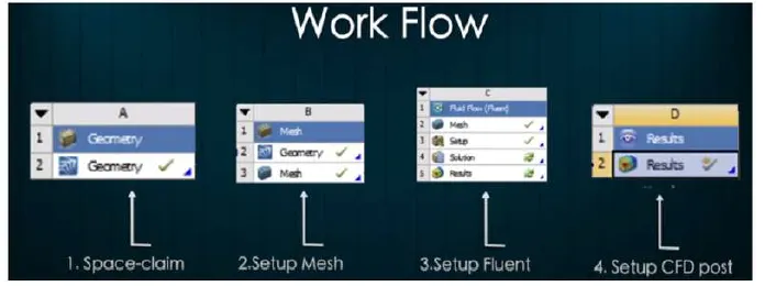
- Geometry: Spaceclaim, where we import geometry.
- Mesh: where boundary naming, element sizing and mesh generation with required grid size will be done.
- Setup: Ansys fluent, where actual case setup will be done.
- Solution: Ansys fluent, where runtime results visualization done.
- Results: CFD-post, where post processing of results will be done.
CAD Import:
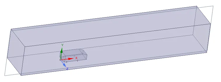
After import Ahmed body we create a computational domain as shown in below figure.
Computational domain are created by enclosed option..Prepare -> Enclosure
Dimension to the computational domain around Ahmed body are as follow-
inlet (left side)= 2m
outlet (right side)= 5m
bottom (symmetry)= 0m
top (symmetry)= 1m
width= 0.5m (on both sides)
Create the planes normal along x, y & z axis.
Mesh generation & refining:-
We want to refine the mesh only in the specific region around the car body instead of refining the entire our domain. So we will create a small box inside which our Ahmed body will be placed.
Dimensions of small box as below-
inlet= 0.5m
outlet= 1m
top= 0.5m
bottom= 0m
width= 0.26m
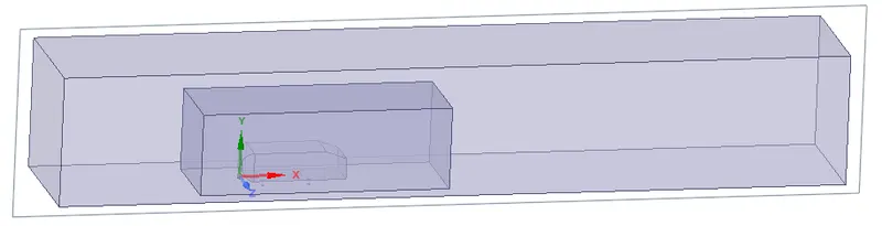
Now generate the mesh to see how baseline mesh (small box and ahmed body) will look like. after this, our computational domain (large box) and baseline mesh (small box) are overlapping, which is undesirable. To merge both boxes, go back to spaceclaim, click plane option, create 3 planes by clickingon the origin. Now select 1st plane and click on "section mode". Now we can see hatching lines inside the small box as crosshatch.

To avoid interference, go to "prepare" and click "right tick" option.
now click on "mode", hide all the planes except "FFF" plane.
Enable only first enslosure.
select 1st plane, click "section mode".
now disable the 1st enclosure & by enabling the second enclosure we can see that our Ahmed body has been hidden.
Click "FFF" plane to see set the "share topology" option as "merge". Then only our both the boxes will share information with each other.
close the window. open mesh again from ansys workbench. Generate the mesh, right click on mesh, click method, select body, hide section plane 1, click apply on geometry.
select method, select multizone, assign element size from 413 mm to 100mm to get evenly size mesh at outer region.
generate the mesh.
there are pillars at the bottom of the ahmed body, in mesh it not fully circles. We need to make them round by set element size 5 mm.
Assign inflation layer due to boundary layer of the body over which flow of air takes place. assign total layer thickness as 23 mm, number of layers 5.
close mesh window.
Fluent setup:-
select K-epsilon turbulent model.
Density-based solver because it gives good compressibility effect.
assign time as steady state solver.
material- air
density= 1.22 kg/m^3
viscosity= 0.0000181 kg/m.s
Boundary condition:-
inlet velocity= 25 m/s
temp.= 300K
outlet= 0 Pa
car-wall= wall (no slip condition)
symmetry= symmetry
CFD Results:-
- select car wall, assign colour variable pressure, click apply.
- Create cut-plane-z to see velocity and pressure profile.
- Create the vector plane in cut-plane-z to see the vector plot.
- To obtain the velocity at 2 different point in the cut-plane-z, create 2 points at some distance along cut-plane-z.
- Now to see this velocities distribution go to insert, select chart, go to data series, assign location as line1.
- on x-axis variable, y (coordinate)
- on y-axis velocity variable, velocity (u).
- same way assign second point at some distance.
Baseline mesh setup:- It is a less refined mesh which use to check the overview of simulation.
Nodes= 8584
Cell counts= 42561
Mesh:

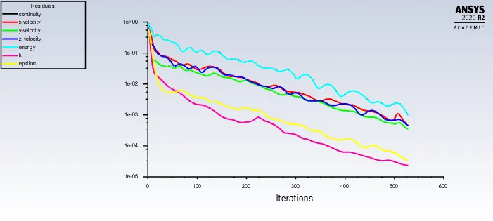
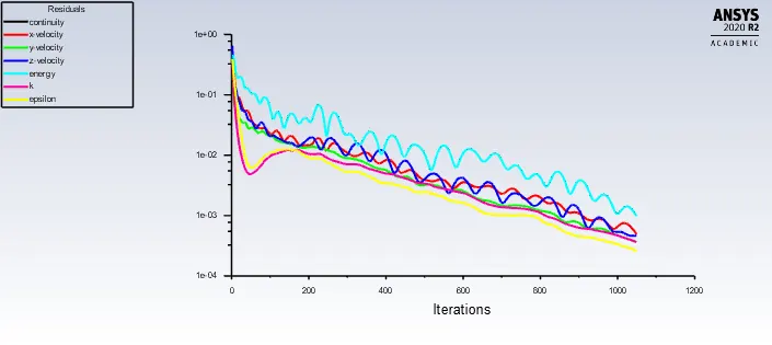
Residuals plot:
Drag Coefficient (cd):
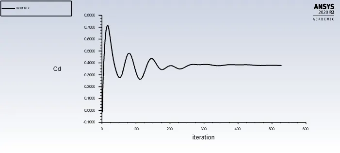
Coeff. of drag (Cd) is 0.378
Lift Coefficient (cl):
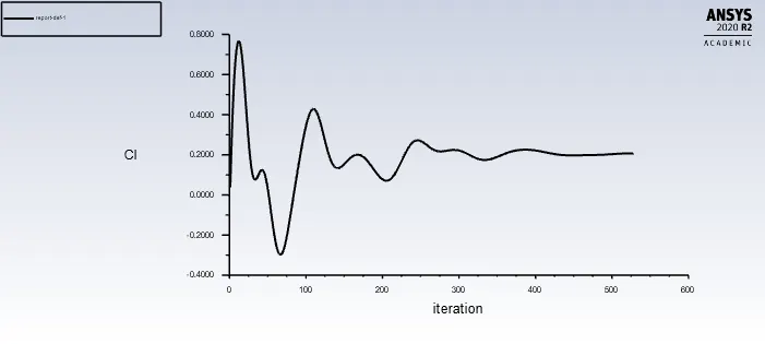
Coeff. of lift (Cl) is 0.206
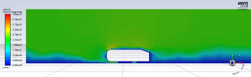
Velocity contour:
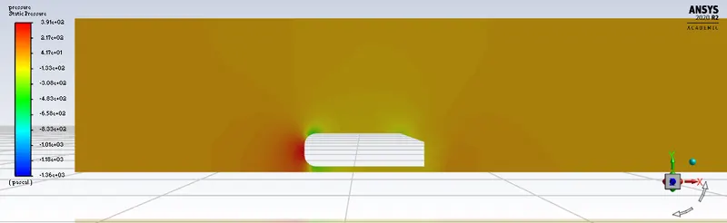
Pressure contour:
Vector plot:
Velocity distribution plot:
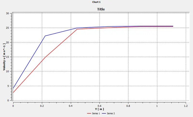
conclusion from velocity distribution plot- From the above plot velocity distribution at 2 lines at some distance from the rear end of Ahmed body, velocity increases as the vertical distance increase because after the velocity loss at rear end of body, it regains its momentum due to rejoining the streamline ( y=0 to 0.8) and further vertical distance shows velocity is constant which represents natural streamline velocity.
---------------------------------------------------------------------------------------------------
Refined mesh setup:
Case 1: Nodes= 29133 Elements= 86487
Mesh element size= 100 mm
Body sizing= 50 mm
Face sizing= 5 mm
Mesh:

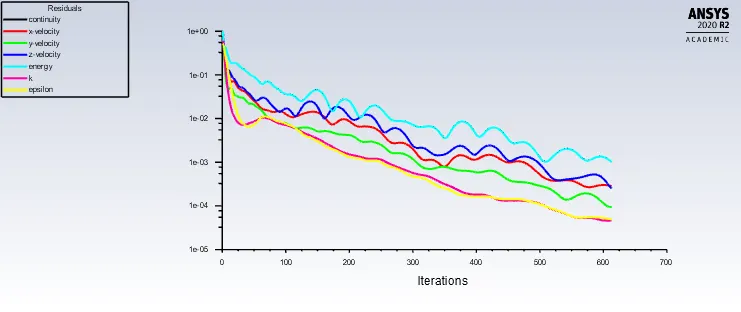
Residuals plot:
Drag Coefficient (cd):
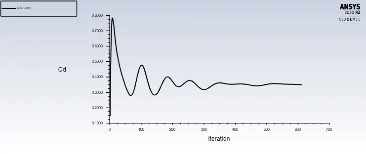
Coeff. of drag (Cd) is 0.349
Lift Coefficient (cl):
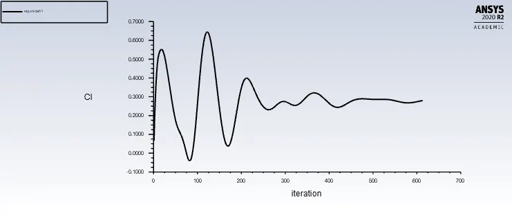
Coeff. of lift (Cl) is 0.279
Velocity contour:
Pressure contour:
Vector plot:
Velocity distribution plot:
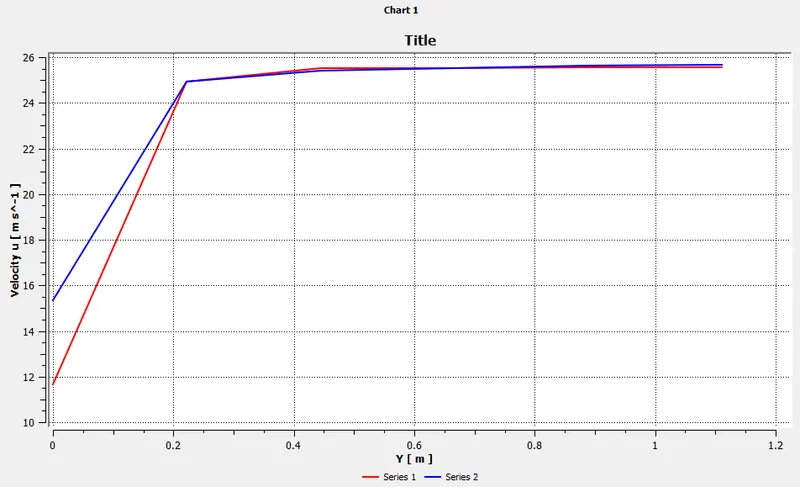
conclusion from velocity distribution plot- From the above plot velocity distribution at 2 lines at some distance from the rear end of Ahmed body, velocity increases as the vertical distance increase because after the velocity loss at rear end of body, it regains its momentum due to rejoining the streamline ( y=0 to 0.42) and further vertical distance shows velocity is constant which represents natural streamline velocity.
Case 2: Nodes=49896 Elements=151066
Mesh element size= 75 mm
Body sizing= 40 mm
Face sizing= 5 mm
Mesh:

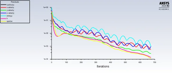
Residuals plot:
Drag Coefficient (cd):
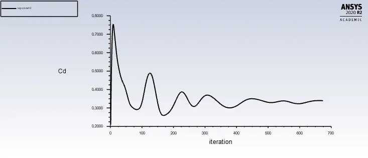
Coeff. of drag (Cd) is 0.339
Lift Coefficient (cl):
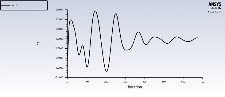
Coeff. of lift (Cl) is 0.311
Velocity contour:
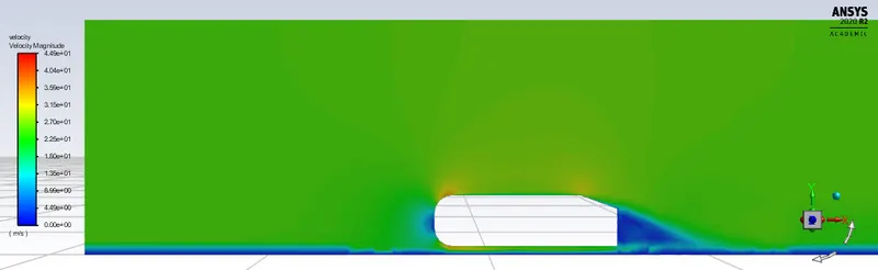
Pressure contour:
Vector plot:
Velocity distribution plot:
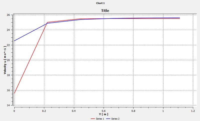
conclusion from velocity distribution plot- From the above plot velocity distribution at 2 lines at some distance from the rear end of Ahmed body, velocity increases as the vertical distance increase because after the velocity loss at rear end of body, it regains its momentum due to rejoining the streamline ( y=0 to 0.42) and further vertical distance shows velocity is constant which represents natural streamline velocity.
Case 3: Nodes=123054 Elements= 357242
Mesh element size= 50 mm
Body sizing= 30 mm
Face sizing= 5 mm
Mesh:

Residuals plot:
Drag Coefficient (cd):
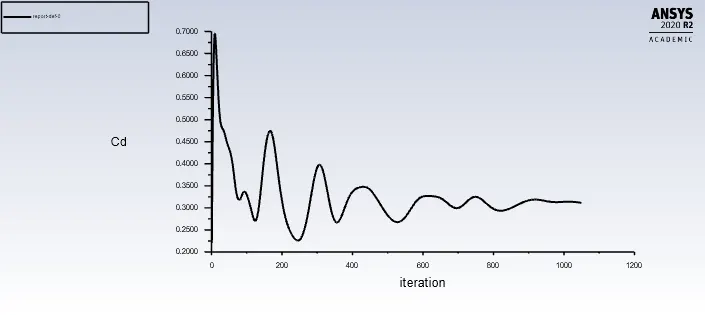
Coeff. of drag (Cd) is 0.311
Lift Coefficient (cl):
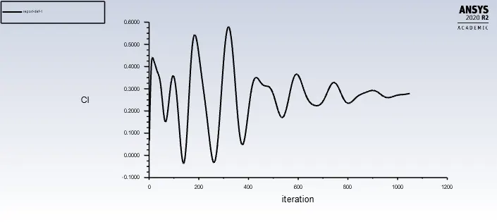
Coeff. of lift (Cl) is 0.278
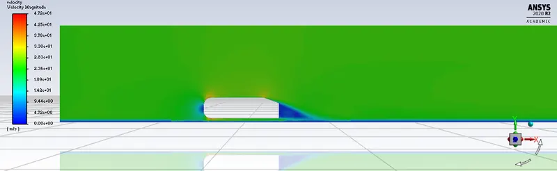
Velocity contour:
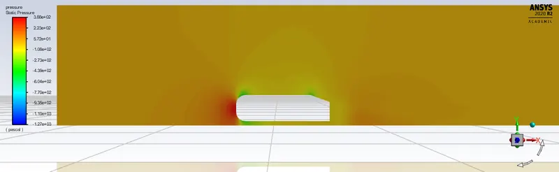
Pressure contour:
Vector plot:
Velocity distribution plot:
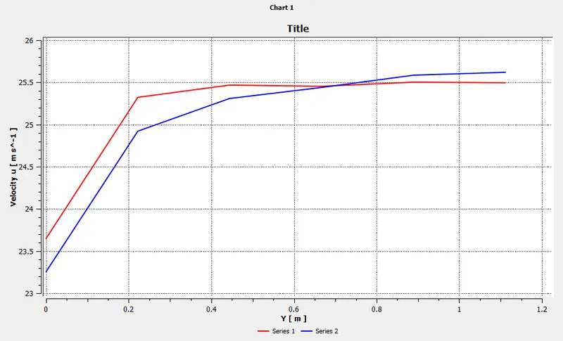
conclusion from velocity distribution plot- From the above plot velocity distribution at 2 lines at some distance from the rear end of Ahmed body, velocity increases as the vertical distance increase because after the velocity loss at rear end of body, it regains its momentum due to rejoining the streamline ( y=0 to 0.35) and further vertical distance shows velocity is constant which represents natural streamline velocity.
Effect of mesh refinement on the coefficient of drag and lift:
| Mesh size (mm) | Body size (mm) | Face size (mm) | Coeff of Drag (cd) | Coeff of Lift (cl) | Nodes | Elements |
| 100 | 50 | 5 | 0.349 | 0.279 | 29133 | 86487 |
| 75 | 40 | 5 | 0.339 | 0.311 | 49896 | 151066 |
| 50 | 30 | 5 | 0.311 | 0.278 | 123054 | 357242 |
Conclusion:
- As we increase number of cells then accuracy of solution also gets increases.
- As we know coeff. of drag is depends on Reynolds number, so by change grid sizes coeff. of drag is not effected.
- As we fine the mesh, then velocity distribution become more accurate.
- By increasing the refinement of mesh, computational times also increase.