Week 9- Unsteady moving zones Approach

Aim: To simulate the motion of blades in a turbomachinery component using an unsteady approach.

Transient simulation:

Transient simulations are performed when the parameters vary with time.

Moving Mesh approach:

• In this approach, the Mesh is moving and the Mesh topology will change that is the mesh shape will vary with the motion of the frame.
• There is a change in the control volume (the region of fluid we need to analyzed).
• It is an unsteady Phenomenon. It can be used on unsteady flows when unsteadiness is the main concern of the simulation.
• This method gives good results for unsteady flows but requires inputting complex boundary conditions.
• This approach is used for modeling unsteady phenomena like vortex-induced flows and if there is an interaction of the vortex with the bodies.

Simulation setup:

• Import the mesh model and select the pressure-based solver and absolute frame of reference.
• Select the solver as a k-epsilon realizable model as it gives the best results for the turbo machinery components and select standard wall treatment.
• Select the cell zone conditions.
• The cell zone conditions for the rotating frame give rotational velocity as 250 rpm and select mesh motion.
• In solution methods for turbulent kinetic energy and turbulent dissipation rate take a second-order upwind method and coupled. set the courant number to 10.
• Define required contours.

Solver Settings:

Solver settings for mesh motion in a turbine
Type:	Pressure-based
Velocity formulation:	Absolute
Time setting:	Transient
Space:	2D
Energy:	OFF
Model:	k-epsilon-realizable, standard wall function
Setup conditions:	fluid-rotor Mesh motion- yes Moving Mesh Rotation Speed [rev/min] 250
Cell Zones	Fixed Frame - Fluid Rotating frame - Fluid Surface body - Fluid
Mesh Interface	Rotor-stator-interface
Boundary conditions:	inlet - pressure inlet outlet - pressure outlet Gauge Total Pressure 0 pa there is no pressure difference in inlet and outlet
Solution methods:	COUPLED
Pressure interpolation scheme:	Second-Order Upwind
Momentum:	Second-Order Upwind
Turbulence:	Second-Order Upwind
Flow courant number	10
Initialization:	Hybrid
The material used, Fluid	Air
Monitor :	Mass flow rate outlet Static pressure contour Velocity contour

Time step calculation for 300 rpm:

`T = 60/N`

T = 0.2

if we want the simulation to be achieved within 1000 time steps then the time period is `DeltaT`= 0.0002

The time step needs to be smaller than this or equal to this to get accurate results.

If the time step is larger the solution may be over estimated or under estimated.

Moving Mesh velocity animation:

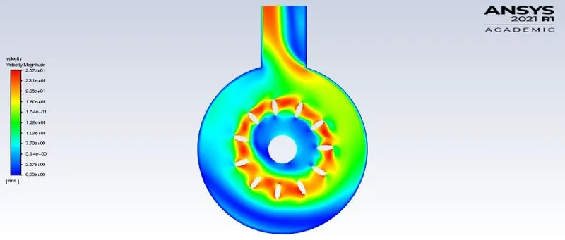
• Stability is attained at a max velocity of 25.7m/s which is also the same in the steady-state simulation.
• velocity of the fluid is high at the rotor as the rotor is rotating at high velocity which makes the fluid to have high velocity.
• The velocity at the inlet is low.
• velocity of fluid is increased near the outlet
• The velocity near the outer walls is zero following the no slip condition.

Moving Mesh Pressure animation:

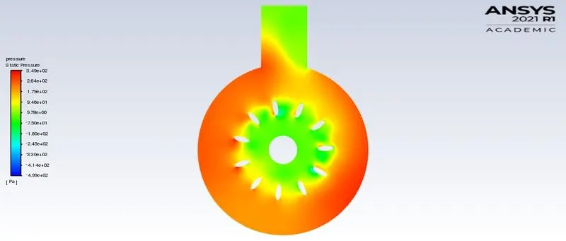
• The pressure at the wall is high
• the pressure at the rotors is low as the pressure energy is converted into kinetic energy.

Mass flow rate at the outlet:

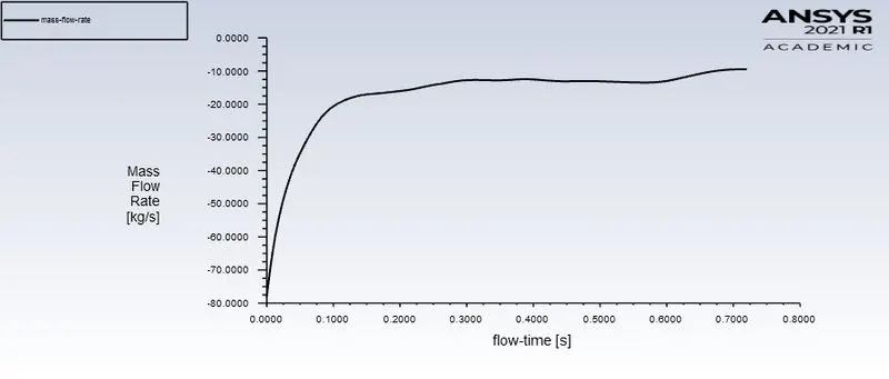
Mass flow rate at the outlet and inlet:

• mass flow rate at the inlet and outlet is same according to the newtons law of conservation of mass
• The negative mass flow rate at the outlet indicates that the flow is leaving the system.
• The Positive mass flow rate at the inlet indicates that the flow is entering the system.

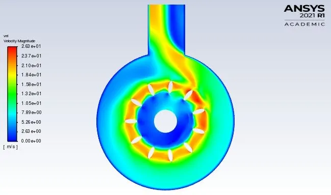
Steady state simulation also performed the contours are as follows

Velocity contour:

Pressure contour:

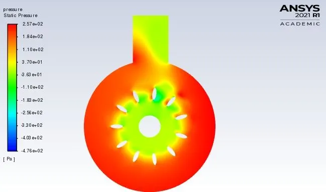
In the transient simulation the velocity and the pressure attained are close.