Week 8- Moving zones approach in Fluent

Aim: To Simulate rotary motion for the provided geometry and plot the velocity profile of the fluid motion. Write about the Moving zones approach.

Introduction:

All the fluid flows that have constant velocity can be easily analyzed, such as an aircraft in cruise mode. To analyze the flow field, we simply change the reference frame to the aircraft and solve the problem as if the air is now flowing around the aircraft at the same constant velocity this makes the simulation easy. However, constant velocity is not always the case in the real world. In ideal conditions, the body might be moving at a constant velocity but Most of the time, moving objects are either accelerating or decelerating. Consider a Badminton shuttlecock moving in the air. Right after it makes contact with the racket, the shuttlecock moves forward and falls (due to gravity). Moreover, in engineering, certain objects undergo rotational acceleration. A perfect example of this is the blades of a helicopter. These blades fixed on the rotor are spinning about the rotor axis at different angular velocities to generate the necessary lift. Turbomachinery offers many such examples where the fluid is undergoing angular acceleration. In both these cases, The fluid analysis cant be performed by assuming the object of concern to be stationary. There are different ways of analyzing the flow field to describe the flow over moving and rotating objects.

Approaches to model zones:

Moving Reference Frame(MRF):

A flow field that is unsteady with respect to the stationary frame becomes steady with respect to the MRF.

• In this approach, the Frame is moving and the Mesh topology will not change that is the mesh shape doesn't vary with the motion of the frame.
• There is no change in the control volume (the region of fluid we need to analyzed).
• It is a Steady Phenomenon. It can be used on unsteady flows when the unsteadiness is not the concern of the simulation.
• A moving reference frame is defined as a reference frame that is in motion with a prescribed orientation and speed with respect to a stationary or inertial reference frame.
• Steady-state problems in the moving frame are easier to solve because of simpler boundary conditions and easier to analyze.
• Reference frames can be used to solve translational and rotational motion, but they are more commonly used for rotational motion problems in turbomachinery applications.

Types of moving reference frames:

Single Moving Reference Frame

Multiple Moving Reference Frame: This type of reference frame uses a mixing plane approach.

• The interface is the region existing in contact between a stationary frame and a moving frame.
• N-S Equations in the stationary frame and rotating frame are solved separately.
• Data is transferred from one frame to the other through the interface.

Methods through which the data is transferred through the interface are

• Area Averaging: `phi_A = 1/AintphidA`
• Mass Averaging:`phi_m = 1/m intrhoVphidA`
• Mixed out approach: This is the best approach as it is most accurate because of no averaging. Solves the continuity, momentum, and energy equations.

Moving Mesh approach:

• In this approach, the Mesh is moving and the Mesh topology will change that is the mesh shape will vary with the motion of the frame.
• There is a change in the control volume (the region of fluid we need to analyzed).
• It is an unsteady Phenomenon. It can be used on unsteady flows when unsteadiness is the main concern of the simulation.
• This method gives good results for unsteady flows but requires inputting complex boundary conditions.
• This approach is used for modeling unsteady phenomena like vortex-induced flows and if there is an interaction of the vortex with the bodies.

Simulation setup:

• Import the mesh model and select the pressure-based solver and absolute frame of reference.
• Select the solver as a k-epsilon realizable model as it gives the best results for the turbo machinery components and select enhanced wall treatment.
• Select the cell zone conditions.
• The cell zone conditions for the rotating frame give rotational velocity as 250 rpm.
• In solution methods for turbulent kinetic energy and turbulent dissipation rate take a second-order upwind method and coupled. set the courant number to 10.
• Define required contours.

Contours From the simulation:

Velocity Contour:

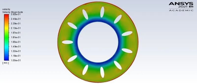
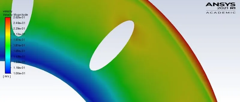
• The velocity of the fluid near the outer walls is high as there is more displacement from the airfoils.
• The velocity of the fluid near the inner walls is very less.

Velocity Vector:

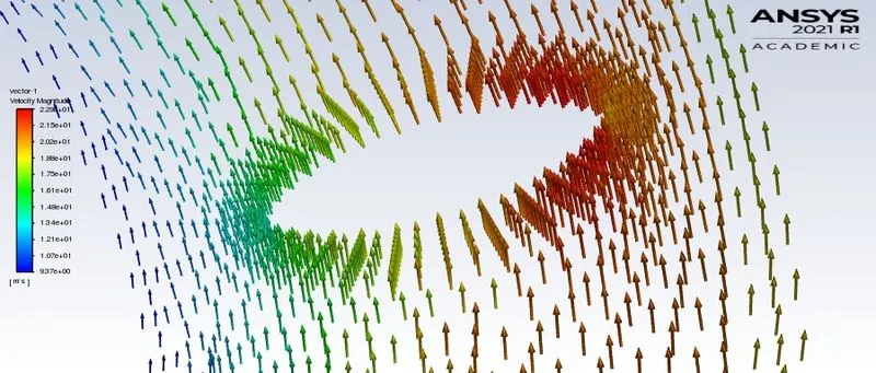
• It can be seen that the velocity of the fluid particles near the top of the airfoil has the highest velocity. There is a slight decrease in the velocity of the fluid particles at the top of the airfoil.

Pressure Contour:

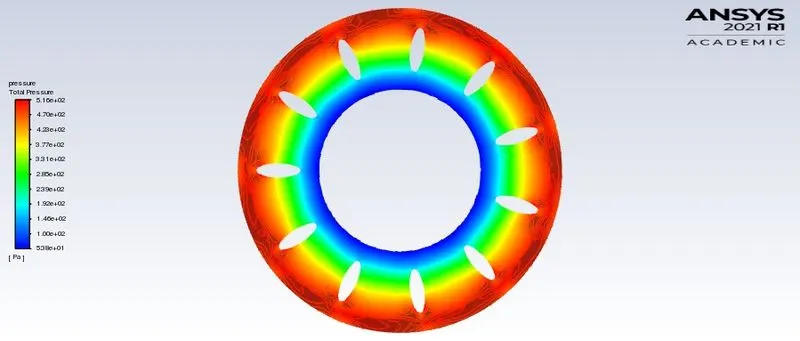
The total pressure is distributed from the lowest pressure at the inner walls and grows towards the outer surface. The lower tip of the airfoil experiences the lowest pressure and the upper tip experiences the highest pressure.

Turbulence contour:

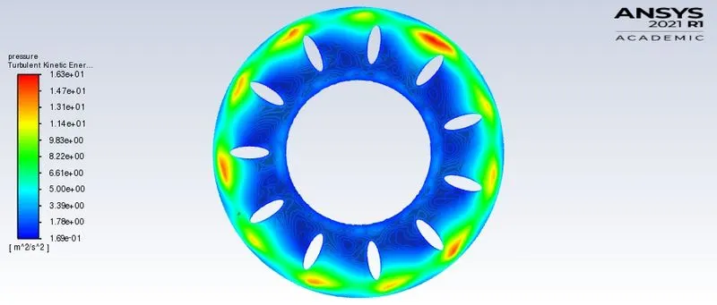
It is seen that there are high turbulence regions formed near the outer surface.