Week 9 - FVM Literature Review
Objective:
- What is the Finite Volume Method(FVM)?
- The major differences between FDM & FVM.
- The need for interpolation schemes and flux limiters in FVM.
Finite Volume Method
The finite volume method (FVM) is a method for representing and evaluating partial differential equations in the form of algebraic equations.
The finite volume method (FVM) is a discretization technique for partial differential equations. FVM uses a volume
integral formulation of the problem with a finite partitioning set of volumes to discretize the equations
In FVM, instead of writing equations at a point, we write it for the entire volume. Finite Volume representation preserves the concept of conservation.
In the finite volume method, volume integrals in a partial differential equation that contain a divergence term are converted to surface integrals, using the divergence theorem. These terms are then evaluated as fluxes at the surfaces of each finite volume.
Steps in FV Discretization
- We write governing equation in its integral form.
- Apply gauss divergence theorem.
- Calculate 'Flux Terms'.
A steady-state heat conduction equation with heat generation.
`(del)/(delx)(alpha*(delT)/(delx)) + S = 0`
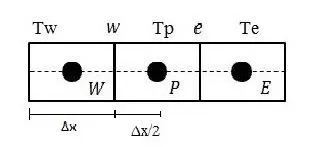
Now, integrating the above equation wrt dv,
`int((del)/(delx)(alpha*(delT)/(delx)) + S) = 0`
`int(del)/(delx)(alpha*(delT)/(delx))dv + intSdv = 0`
`int(del)/(delx)(alpha*(delT)/(delx))A*dx + intSdv = 0`
{dv = A*dx)
`[alphaA(delT)/(delx)]_w^e + barSdv = 0`
`alpha_eA(delT)/(delx_e) - alpha_wA(delT)/(delx_w) + barSdv = 0`
`alphaA[(T_e - T_p)/(Deltax)] - alphaA[(T_p - T_w)/(Deltax)] + barSdv = 0`
where, `alphaA[(T_e - T_p)/(Deltax)]` is `[Heat Flux]_(out)`
`alphaA[(T_p - T_w)/(Deltax)]` is `[Heat Flux]_(i n)`
`barSdv` is Source Term
The amount of heat removed is conserved.
Differences between FDM & FVM
We cannot use FDM when the grids are not aligned along x, y, and z-direction.
We can use FVM for the entire volume to solve our problem.
Interpolation schemes in FVM
Interpolation is a process to estimate the values at unknown points by using the points with known values and sample points on either side of the unknown point. In FVM, interpolation schemes are used to find values of volume integrals required at points other than nodes.
Example: consider the simple case of steady one-dimensional convection and diffusion.
`(d)/(dx)(rhouphi) = (d)/(dx)(tau(dphi)/(dx))`
where, `phi` is our solution variable, `rho` is density, `u` is velocity, `tau` is diffusion coefficient.
Integration of this governing equation over control volume,
`(rhouphi)_e - (rhouphi)w = (tau(dphi)/(dx))_e - (tau(dphi)/(dx))_w`
Different types of interpolation schemes are:
- Upwind Interpolation Scheme (UDS)
- Linear Interpolation Scheme
- Quadratic upwind Interpolation Scheme
- Hybrid Interpolation Scheme
- Total variation Diminishing Scheme
The Upwind interpolation scheme takes into account the direction of fluid flow and based on it, the value of the solution variable at the face is approximated by its value at the upstream computational node.
Flux Limiters
For convective fluid flow, it is observed that the low-order schemes are usually stable but quite dissipative in nature around the points of discontinuity or shocks while the higher-order schemes are unstable in nature and show oscillations in the vicinity of discontinuity or shocks. Highly accurate and oscillation-free schemes are known as High-Resolution Schemes.
Flux Limiter functions are used to fine-tune the higher order and lower order schemes in such a way that the resulting scheme gives a higher-order accuracy in the smooth region of the flow and maintains first-order accuracy in the vicinity of shocks and discontinuities. For such a scheme TVD scheme is employed.
Consider 1D semi dicrete scheme,
`F(u_(i+1/2)) = f_(i+1/2)^(low) - phi(r_i)(f_(i+1/2)^(low) - f_(i+1/2)^(high))`
`F(u_(i+1/2)) = f_(i-1/2)^(low) - phi(r_i)(f_(i-1/2)^(low) - f_(i-1/2)^(high))`
where,
`f^(low)` is low precision flux
`f^(high)` is high precision flux
`phi(r)` Flux limiter function
The `psi(r)` represnts the flux limiter function,
`F_e = L_e + psi(r)(H_e - L_e)`
Flux limiters function depends upon the smoothness parameter r which is defined as,
`r_p = (phiP -phiW)/(phiE -phiP)`