Week 7 - Auto ignition using Cantera
AUTO IGNITION USING CANTERA
Objective
To detrmine auto ignition and ignition delay time for methane combustion reaction for various conditions.
Part 1
- variation of Auto Ignition time of Methane with a constant temperature of 1250K and pressure varying from 1 to 5 atm.
- variation of Auto Ignition time of Methane with a constant pressure of 5 atm and temperature varying from 950K to 1450K.
part 2
observe and print the rate of change of molar concentrations of the given elements "H2O, O2, OH" with respect to the time, (simulation time = 10 secs)
Explain the behavior of the graph for 2 cases,
- When Temperature is 1000K and pressure 5 bar
- When Temperature is 500K and pressure 5 bar
Auto Ignititon:
Autoignition occurs when a mixture of gases or vapors ignites spontaneously with no external Ignition source and after reaching a certain temperature, the autoignition temperature.The autoignition temperature is not an intrinsic property of the gases or vapors but is the lowest temperature in a system where the rate of heat evolved from the gases or vapors increases beyond the rate of heat loss to the surroundings, resulting in the Ignition. . The autoignition time decreases exponentially with increasing unburned mixture temperature, and approximately linearly with increasing pressure.
Auto Ignition temperature can be affected by the pressure, vessel shape and volume, contaminants, surface activity, reaction rate, gravity, etc.
Ignition Delay:
the time interval between the start of injection and the start of combustion. This delay period consists of (a) physical delay, wherein atomization, vaporization, and mixing of air-fuel occur and (b) of chemical delay attributed to pre-combustion reactions. Physical and chemical delays occur simultaneously. To reduce NOx, the method adopted in modern engines is to reduce the ignition delay.
For predicting heat release in modern engines, therefore, the estimation of ignition delay is no more important. However, the ceiling on NOx is dipping to such a low level that accurate prediction of ignition delay has become important even if it is small.
Calculating Ignition Delay:
Time ignition Delay = IntialTemperature + 400K
Part 1
- variation of Auto Ignition time of Methane with a constant temperature of 1250K and pressure varying from 1 to 5 atm.
Code:
import cantera as ct
import matplotlib.pyplot as plt
import numpy as np
#####
gas=ct.Solution('gri30.xml')
T=1250
Pressure=np.linspace(1,5,5)
ig=[]
for P in Pressure:
     gas.TPX=T,P*101325,{'CH4':1,'O2':2,'N2':7.52}
#defins the governing egqns to be solved
     r=ct.IdealGasReactor(gas)
     sim=ct.ReactorNet([r])
     time=0
     states=ct.SolutionArray(gas,extra=['time_ms','t'])

     T_old=T


     for n in range(10000+1):
         time+=1e-3
         sim.advance(time)
         states.append(r.thermo.state,time_ms=time*1e-3,t=time)


         T_new=states.T
         T_new=T_new[n-1]
         if (T_new> 400+T_old):
             ig.append(time)
         T_old=states.T
         T_old=T_old[n-1]
     plt.figure(1)
     plt.plot(states.t, states.T)
     plt.xlabel('time (ms)')
     plt.ylabel('temperature')


plt.figure(2)
plt.plot(Pressure,ig)
plt.xlabel('pressure (atm)')

plt.ylabel('ignition delay (ms)')
plt.show()
Plots:
Temperature v/s time
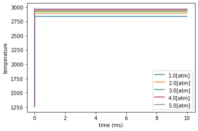
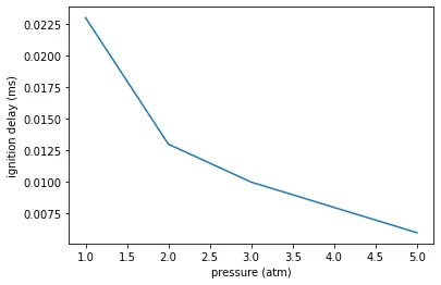
since Pressure is directly proprtional to Temperature in ideal gas condition.With increasing pressure,Temperature is increased.that is from plot below Variation of Pressure with Ignition delay by increasing Pressure in the system the ignition delay decreases
- variation of Auto Ignition time of Methane with a constant pressure of 5 atm and temperature varying from 950K to 1450K.
import cantera as ct
import matplotlib.pyplot as plt
import numpy as np
#####
gas=ct.Solution('gri30.xml')
P=5
temperature=np.linspace(950,1250,5)
ig=[]
for T in temperature:
     gas.TPX=T,P*101325,{'CH4':1,'O2':2,'N2':7.52}
#defins the governing egqns to be solved
     r=ct.IdealGasReactor(gas)
     sim=ct.ReactorNet([r])
     time=0
     states=ct.SolutionArray(gas,extra=['time_ms','t'])

     T_old=T


     for n in range(10000+1):
         time+=1e-3
         sim.advance(time)
         states.append(r.thermo.state,time_ms=time*1e-3,t=time)


         T_new=states.T
         T_new=T_new[n-1]
         if (T_new> 400+T_old):
             ig.append(time)
         T_old=states.T
         T_old=T_old[n-1]
     plt.figure(1)
     plt.plot(states.t, states.T)
     plt.xlabel('time (ms)')
     plt.ylabel('Temperature')
     plt.legend([str(T)+'[k]' for T in temperature])


plt.figure(2)
plt.plot(temperature,ig)
plt.xlabel('temperature (k)')

plt.ylabel('ignition delay (ms)')
plt.show()
Plots:
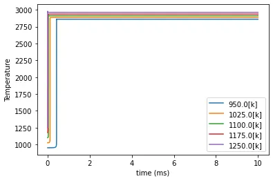
Temperature v/s time
Variation of temperature under constant pressure
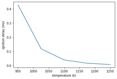
ignition delay v/s temperature
As temperature increases ignition delay decreases and vice-versa
part 2
observe and print the rate of change of molar concentrations of the given elements "H2O, O2, OH" with respect to the time, (simulation time = 10 secs)
Explain the behavior of the graph for 2 cases,
- When Temperature is 1000K and pressure 5 bar
Code:
import cantera as ct
import matplotlib.pyplot as plt
#####
gas=ct.Solution('gri30.xml')
####
def igdelay(T,P):
    gas.TPX=T,P*101325,{'CH4':1,'O2':2,'N2':7.52}
#defins the governing egqns to be solved
    r=ct.IdealGasReactor(gas)
    sim=ct.ReactorNet([r])
    time=0.0

    states=ct.SolutionArray(gas,extra=['time_ms','t'])
    for i in range(10000+1):
        time+=1e-3
        sim.advance(time)
        states.append(r.thermo.state,time_ms=time*1e-5,t=time)

    #print(states.T)
    #print(states.t)
    plt.figure(1)

    plt.plot(states.t,states('oh').Y, color='b')
    plt.xlabel('time in ms')
    plt.ylabel('molefraction of OH')

    plt.figure(2)

    plt.plot(states.t,states('H2O').Y, color='r')
    plt.xlabel('time in ms')
    plt.ylabel('molefraction of H2O')


    plt.figure(3)

    plt.plot(states.t,states('O2').Y, color='g')
    plt.xlabel('time in ms')
    plt.ylabel('molefraction of O2')

    plt.show()

igdelay(1000, 5)
Results and plots:
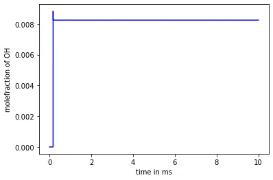
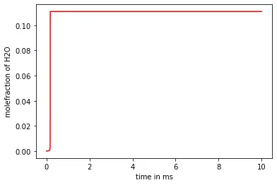
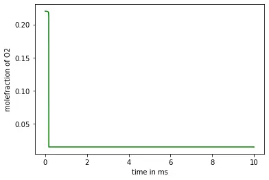
When Temperature is 500K and pressure 5 bar
using above code and calling the function "igdelay(Temperature,pressure)"
igdelay(500, 5)
plots:
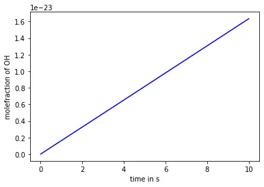
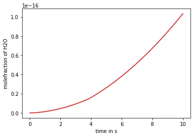
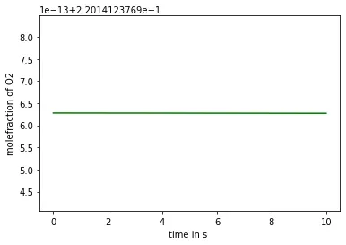
Now comparing the 1000k,5bar and 500k,5 bar plots:
We can see a drastic difference between them.Since the initial temperature was very low for 500k plots.there the complete combustion can't be observed.Since auto ignition temperature of methane is around 875k ,comparing to 500k this is a huge margin.In O2 plots
for 1000k for 500k
from these plots we can observe the O2 molefraction for 500k is constant"this is proves that oxygen bonds are not broken in 500k since breaking the double bond in O2 require more energy.while in 100ok we can see the complete oxidization.
for OH plots:
for 1000k for 500k
comparing these plots for OH,for 1000k plot the OH has been produced and achieved equilibrium or stabilized.but in case of 500k we can see an increase in molefraction but not stabilized this is because the energy is spend on breaking OH and H20 bonds,or in the reaction process.
for 1000k for 500k
References