Week 5.2 - Literature review: ODE Stability

ODE STABILITY

Objective

Literature review of ODE stability

Theory

Numerical solution schemes are often referred to as being explicit or implicit. When a direct computation of the dependent variables can be made in terms of known quantities, the computation is said to be explicit. When the dependent variables are defined by coupled sets of equations, and either a matrix or iterative technique is needed to obtain the solution, the numerical method is said to be implicit.

In computational fluid dynamics, the governing equations are nonlinear, and the number of unknown variables is typically very large. Under these conditions implicitly formulated equations are almost always solved using iterative techniques.

Iterations are used to advance a solution through a sequence of steps from a starting state to a final, converged state. This is true whether the solution sought is either one step in a transient problem or a final steady-state result. In either case, the iteration steps resemble a time-like process. Of course, the iteration steps usually do not correspond to a realistic time-dependent behavior. In fact, it is this aspect of an implicit method that makes it attractive for steady-state computations, because the number of iterations required for a solution is often much smaller than the number of time steps needed for an accurate transient that asymptotically approaches steady conditions.

Stability, in mathematics, condition in which a slight disturbance in a system does not produce too disrupting an effect on that system. In terms of the solution of a differential equation, a function f(x) is said to be stable if any other solution of the equation that starts out sufficiently close to it when x = 0 remains close to it for succeeding values of x. If the difference between the solutions approaches zero as x increases, the solution is called asymptotically stable. If a solution does not have either of these properties, it is called unstable.

Stability of solutions is important in physical problems because if slight deviations from the mathematical model caused by unavoidable errors in measurement do not have a correspondingly slight effect on the solution, the mathematical equations describing the problem will not accurately predict the future outcome.

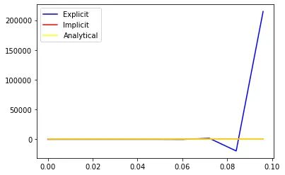
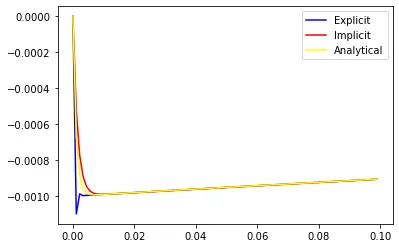
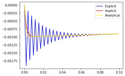
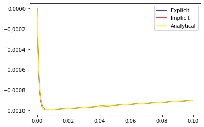
The principal reason for using implicit solution methods, which are more complex to program and require more computational effort in each solution step, is to allow for large time-step sizes.

generally

import numpy as np
import matplotlib.pyplot as plt

def explicit_euler(total_t,dt):
    t=np.arange(0,total_t,dt)
    y=np.zeros(len(t))
    
    for i in range(1,len(t)):
        y[i]=y[i-1]+dt*(-1000*y[i-1]-np.exp(-t[i-1]))
    
    return [t,y]

def implicit_euler(total_t,dt):
    t=np.arange(0,total_t,dt)
    y=np.zeros(len(t))
    
    for i in range(1,len(t)):
        y[i]=(y[i-1]-np.exp(-t[i-1])*dt)/(1+1000*dt)
    
    return [t,y]
def analytical_euler(total_t,dt):
    t=np.arange(0,total_t,dt)
    y=np.zeros(len(t))
    
    for i in range(1,len(t)):
        y[i]=np.exp(-1000*t[i])*(1-np.exp(999*t[i]))/999
    return y
        
    

total_t=0.1
dt=1e-4
t,y_explicit=explicit_euler(total_t, dt)
t,y_implicit=implicit_euler(total_t, dt)
y_analytical=analytical_euler(total_t, dt)
plt.plot(t,y_explicit,color='blue')
plt.plot(t,y_implicit,color='red')
plt.plot(t,y_analytical,color='yellow')
plt.legend(['Explicit','Implicit','Analytical'])
plt.show()