Week 6 - Multivariate Newton Rhapson Solver

AIM: To solve the give set of Ordinary differential equations using Multivariate Newton-Raphson Method

Theoritical Background:

Newton-Raphson Iteration

Let f(x) be a well-behaved function, and let r be a root of the equation f(x) = 0. Of the many iterative root-finding procedures, the Newton-Raphson method, with its combination of simplicity and power, is the most widely used.

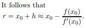
Let x₀ be a good estimate of 'r' and let r = x₀ + h. Since the true root is 'r', and h = r − x₀, the number 'h' measures how far the estimate x₀ is from the truth. Since h is ‘small,’ we can use the linear (tangent line) approximation to conclude that

and therefore, unless f ‘ (x₀) is close to 0,

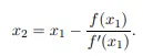
The next estimate x₂ is obtained from x₁ in exactly the same way as x₁ was obtained from x₀:

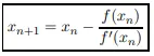
If x_n is the current estimate, then the next estimate x_n+1 is given by

Given Differential Equations

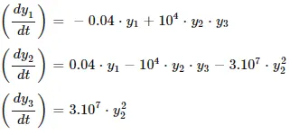
For a coupled Ordinary differential equation with multiple variables We need to modify the solver by incorporating column matrices for the guess values and function values. According to Multivariate Newton-Raphson method to get the solution out of coupled non-linear Ordinary differntial equation below equation is used

α --- relaxation factor

J- Jacobian Matrix

F - Function value at new time step size

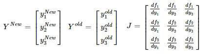
To convert the differential equation in to non-linear equation we are using Backward differencing method

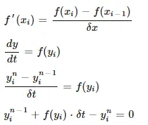
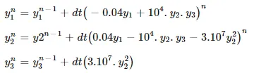
Using Backward differencing scheme we can rewrite the differential equation as

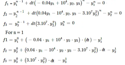
RHS - LHS

Python Code:

"""
Program to solve the system of ODE
dy1/dt = -0.04y1 + 10^4 y2.y3
dy2/dt = 0.04y1 - 10^4 y2.y3 - 3.10^7 y2^2
dy3/dt = 3.10^7 y2^2
"""

import numpy as np 
from numpy.linalg import inv


# Function definition

def f1(y1_old,y1,y2,y3,dt):  # First Non-linear equation
	return(y1_old + dt*(-0.04*y1+pow(10,4)*y2*y3)-y1)

def f2(y2_old,y1,y2,y3,dt):  # Second Non-linear equation
	return(y2_old + dt*(0.04*y1-pow(10,4)*y2*y3 -3*pow(10,7)*pow(y2,2)-y2))

def f3(y3_old,y1,y2,y3,dt):  # Third Non-linear equation
	return(y3_old + dt*(3*pow(10,7)*pow(y2,2))-y3)


# Function to calculate Jacobian Matrix

def Jacobian(y1_old,y2_old,y3_old,y1,y2,y3,dt):

  J= np.zeros((3,3))
  dy = 1e-4
  #Row 1
  J[0,0] = (f1(y1_old,y1+dy,y2,y3,dt)-f1(y1_old,y1,y2,y3,dt))/dy
  J[0,1] = (f1(y1_old,y1,y2+dy,y3,dt)-f1(y1_old,y1,y2,y3,dt))/dy
  J[0,2] = (f1(y1_old,y1,y2,y3+dy,dt)-f1(y1_old,y1,y2,y3,dt))/dy

  #Row 2 
  J[1,0] = (f2(y2_old,y1+dy,y2,y3,dt)-f2(y2_old,y1,y2,y3,dt))/dy
  J[1,1] = (f2(y2_old,y1,y2+dy,y3,dt)-f2(y2_old,y1,y2,y3,dt))/dy
  J[1,2] = (f2(y2_old,y1,y2,y3+dy,dt)-f2(y2_old,y1,y2,y3,dt))/dy

  #Row 3
  J[2,0] = (f3(y3_old,y1+dy,y2,y3,dt)-f3(y3_old,y1,y2,y3,dt))/dy
  J[2,1] = (f3(y3_old,y1,y2+dy,y3,dt)-f3(y3_old,y1,y2,y3,dt))/dy
  J[2,2] = (f3(y3_old,y1,y2,y3+dy,dt)-f3(y3_old,y1,y2,y3,dt))/dy

  return J

# Initial Guess value column Matrix
y_old = np.zeros((3,1))

y_old[0] = 1
y_old[1] = 0
y_old[2] = 0

y_new=y_old


#function column Matrix 

F = np.copy(y_old)
tol = 5e-6
dt = 1e-2
t = np.arange(0,36000,dt)

error = 9e9
alpha = 1
iter = 1

for i in range(0,len(t)):
	while(error>tol):
		F[0] = f1(y_old[0],y_new[0],y_new[1],y_new[2],dt)
		F[1] = f2(y_old[1],y_new[0],y_new[1],y_new[2],dt)
		F[2] = f3(y_old[2],y_new[0],y_new[1],y_new[2],dt)

		J = Jacobian(y_old[0],y_old[1],y_old[2],y_new[0],y_new[1],y_new[2],dt)

		y_new = y_old - alpha*np.matmul(inv(J),F)
		error = np.max(np.abs(y_new-y_old))
		print('Error = {0}'.format(error))
		y_old = y_new
	print('The values of y1={0} y2={1} y3={2} at iteration ={3}'.format(y_new[0],y_new[1],y_new[2],iter))
	iter = iter + 1
	error = 9e9

Results:

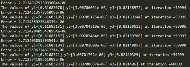
y1 = 0.616, y2 = 3.01e-6 y3 = 0.821

For Implicit method numerical solution is stable even at larger values of time step. With increase in time step size the results obtained vary significantly in terms of accuracy.