Week 6: Conjugate Heat Transfer Simulation
Aim:
To setup the case and perform conjugate heat transfer simulation for flow through the pipe using converge.
Objective:
- Inlet reynolds number is equal to 7000.
- Run grid dependence test on 3 grids and show that the outlet temperature converges to a particular value.
- Set supercyle stage interval to 0.01,0.02 and 0.03
- Add Y+ to your post.in file and Turbulence modelling - K-Epsilon
Intoduction :
Conjugate heat transfer analysis:
CHT is used to describe process where the variation of temperature in both the fluid and the solid due to the thermal interaction between the solid and the fluid.In simple terms it is a combination of the heat transfer in solid and the heat transfer in the fluid.Heat Transfer in solid is conduction whereas heat transfer in fluid in convection.Application like cooling process of the electrical and mechanical component etc.
Super cycling:
Super-cycling is a method used by CONVERGE Studio in the case of conjugate heat transfer problems with solid and liquid regions.The integral problem here is that both solvers cannot run at the same speed since solving in the fluid domain is much faster owing to the time scale difference for heat transfer in liquids as compared to solids. This causes problems during the solution given that the solid side solver would not have reached a steady-state/convergence in the time the liquid solver does. This is where the concept of super-cycling can be used.The basic idea of super-cycling is that the solver for the fluid domain is paused until the solver for the solid domain converges.
Calculating velocity at inlet whose reynolds number is 7000
Re = (rho*V*d)/(Dynamic viscosity)
where,
rho-density of fluid (air)
V-velocity of fluid (air)
d-characteristic length (inner diameter of pipe)
V = (7000*1.849e-5)/(1.184*0.015) = 7.2877 m/s
Velocity = 7.2877 m/s
Case setup:
Boundary Conditions:
Inlet:
Boundary type = inflow
Pressure = zero gradient (Neumann boundary condition)
Temperature = 300 K
Velocity = 7.2877 m/s
outlet:
Boundary type = outflow
Pressure = 101325 Pa
Temperature = 300 K
Species = air
Solid outer wall
Boundary type = wall with slip condition
Wall motion type = stationary
Temperature = -10000 w/m2 (Heat flux)
Solid side
Boundary type = wall with slip condition
Wall motion type = stationary
Temperature = zero gradient (Neumann boundary condition)
Interface
Boundary type = interface
Boundary type = interface
region 1 = Fluid region
Stream ID = 0
Temperature = 300 K
Pressure = 101325 Pa
Species = air
region 2 = Solid region
Stream ID = 1
Temperature = 300 K
Solid option - enabled
Species = Aluminium
Boundary type = interface
region 1 = Fluid region
Stream ID = 0
Temperature = 300 K
Pressure = 101325 Pa
Species = air
region 2 = Solid region
Stream ID = 1
Temperature = 300 K
Solid option - enabled
Species = Aluminium
Geometry:
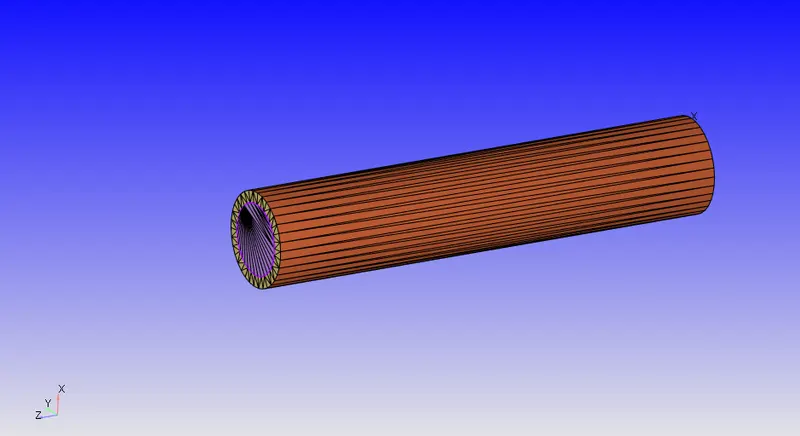
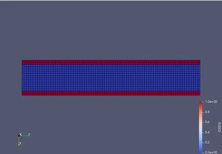
Case 1:
Base grid size - 2.5 mm
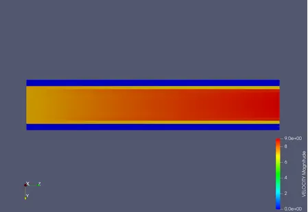
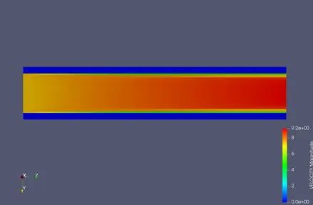
Velocity Contour:
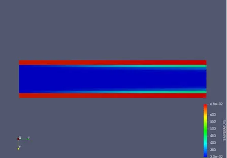
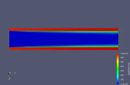
Temperature Contour:
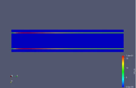
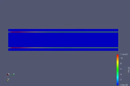
Y Plus:
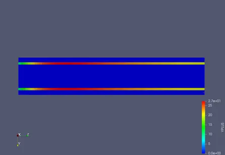
Case 2:
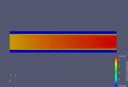
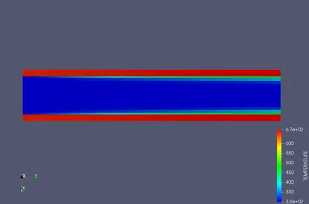
Base grid size - 2 mm
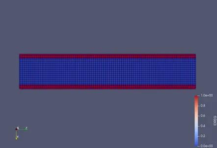
Velocity Contour:
Temperature Contour:
Y plus:
Case 3:
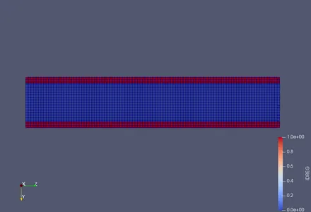
Base grid size - 1.5 mm
Velocity Contour:
Temperature Contour:
Y plus:
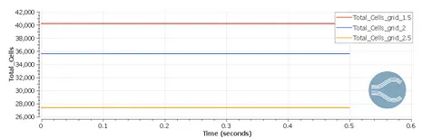
Cell count:
Conclusion:
Mesh refinement has to be done to get grid independant temperature values as slight variation is observed in the mean temperature values of solid region and fluid region for different grid size. The y-plus value decreases as the cell size near the wall is decreased.As we decrease the mesh size there is also drop-in solid region temperature