Week 7: Shock tube simulation project
Objective:
- To Setup a transient shock tube simulation.
- To Plot the pressure and temperature history in the entire domain.
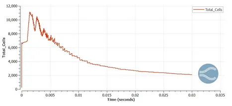
- To Plot the cell count as a function of time .
Introduction:
Shock tube:
The shock tube is a simple duct closed at both end.It consists of two compartments called as driver (high pressure) & driven (low pressure)sections this compartment is separated by metal diaphragm.A high pressure gas reservoir is connected with the driver section.However a vacuum pump is connected to the driven section to maintain driven section pressure.Pressure sensors are generally mounted along the driven tube for pressure measurement.A simple shock tube is a tube, rectangular or circular in cross-section, usually constructed of metal, in which gas at low pressure and gas at high pressure is separated using some form of a diaphragm. The diaphragm suddenly bursts open under predetermined conditions to produce a wave propagating through the low-pressure section. The shock that eventually forms increases the temperature and pressure of the test gas and induces a flow in the direction of the shock wave.By slowly increasing the driver gas pressure for a given driven pressure until the diaphragm gets burst,this bursting of diaphragm creates a compression waves which propagates in the driven section.In a short interval of time,this compression waves merge to form shock wave which propagates in the driven section.Due to arrival of this shock waves in driven section raises the pressure and temperature of stationary low pressure driven gas.At the same time driver gas encounters the expansion due to expansion waves.
Geometry:
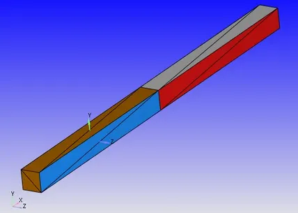
Case setup
Species - O2, N2
Solver - Transient Flow
Navier- stokes solver type: Density-based
Simulation mode -Full hydrodynamic
Gas flow solver - Compressible
Boundary conditions
All the boundaries are given as stationary wall BC (Slip BC) and Two D
Regions
The regions are divided into high pressure and low pressure region
High pressure
- Species: N2
- Pressure=600000 Pa
- Temperature=300K
Low pressure
- Species: O2
- Pressure=101325 Pa
- Temperature=300K
Events

An event is created for simulating the bursting diaphragm, In the beginning, the high pressure and low-pressure regions are closed. After 0.001s the diaphragm breaks and mixing takes place.
Simulation time parameters
Start time=0 s
End time=0.003 s
Initial time step= 1e-9 s
Minimum time step= 1e-9 s
Maximum time step= 1s
Output files
The time interval for writing 3D output files=1e-5 s
So the solver writes a 3D output files after every 1e-5 seconds.
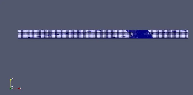
Mesh:
Base grid =0.001 m
The AMR is based on N2 species with an embedding level of 3.sgs-0.001
Post processing results:
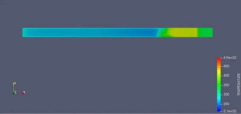
Temperature contour:
Pressure contour:
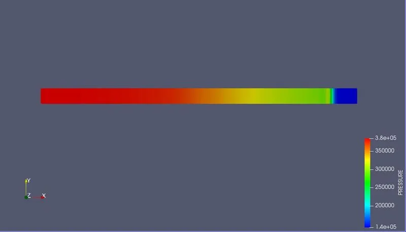
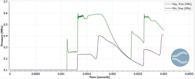
The diaphragm get burst it pushes the N2 gas into the low pressure region but as soon as this N2 gas reaches the end of the shock tube,the reflected shock waves pushes it into the opposite direction which is in high pressure region this wave is again reflected from the other end of the tube pushing the N2 gases in opposite direction.
Temperature:
Pressure:
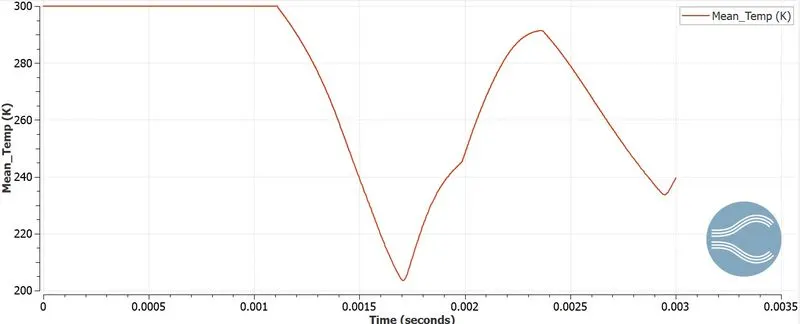
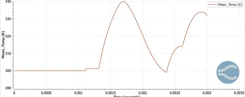
At the beggining, the expansion of the driver gas (N2) creates an important decrease in its temperature, and the other way around for the driven gas (O2). After the waves reflection, the recirulation zone creates again a temperature change in the two zones.
Total cell count:
Animation link:
https://drive.google.com/file/d/1E8R-_uAYN6sw0o9KvGYy7C_AIb3dENFo/view?usp=sharing
When the diaphragm bursts, driver gas rushes to the low-pressure region (driven gas) The bursting diaphragm produces a series of pressure waves, each increasing the speed of sound behind them so that they compress into a shock propagating through the driven gas. This shock wave increases the temperature and pressure of the driven gas and induces a flow in the direction of the shock wave