Rayleigh Taylor Instability Challenge

Objectives:

• Practical CFD models and calculations that are based on the mathematical analysis of Rayleigh Taylor waves .
• To perform the Rayleigh Taylor instability simulation for 2 different mesh sizes with the base mesh being 0.5 mm and compare the results .
• To perform simulation with water and user defined material for a refined mesh (density = 400 kg/`m^3` and viscosity = 0.001kg/m-s).

Types of Instability and some practical CFD models that have been based on the mathematical analysis of Rayleigh Taylor waves:

Kelvin–Helmholtz instability:

can occur when there is velocity shear in a single continuous fluid, or where there is a velocity difference across the interface between two fluids. An example is a wind blowing over water: The instability manifests in waves on the water surface. More generally, clouds, the ocean, Saturn's bands, and the sun's corona show this instability.

Ritchmyer-Meshkov instability:

The Richtmyer–Meshkov instability (RMI) occurs when two fluids of different density are impulsively accelerated. Normally this is by the passage of a shock wave.It combines compressible phenomena, such as shock interaction and refraction, with hydrodynamic instability, including nonlinear growth and subsequent transition to turbulence, across a wide range of Mach numbers.

Plateau–Rayleigh instability:

The Plateau–Rayleigh instability, often just called the Rayleigh instability, explains why and how a falling stream of fluid breaks up into smaller packets with the same volume but less surface area. This fluid instability is exploited in the design of a particular type of ink jet technology whereby a jet of liquid is perturbed into a steady stream of droplets.

Geometry Creation:

• The geometry was created in spaceclaim as square boxes using the rectangle sketch tool.
  
• Then it is converted into surface using Pull tool and share topology is turned on with 1 edge as common.
  
• The surface model was further processed for meshing and the results were taken for three different meshing schemes.

Cases:

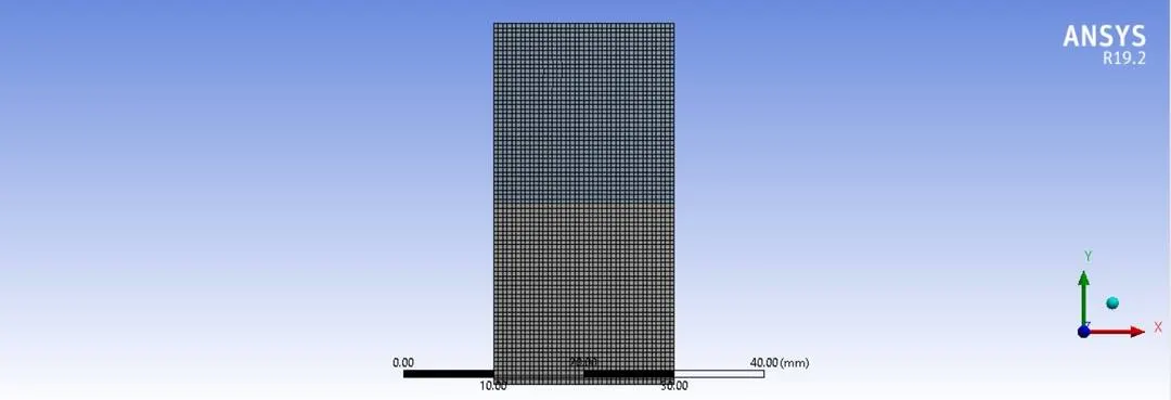
• Case 1. Mesh details: Baseline mesh-0.5mm Element size, Elements –3200, Nodes –332.
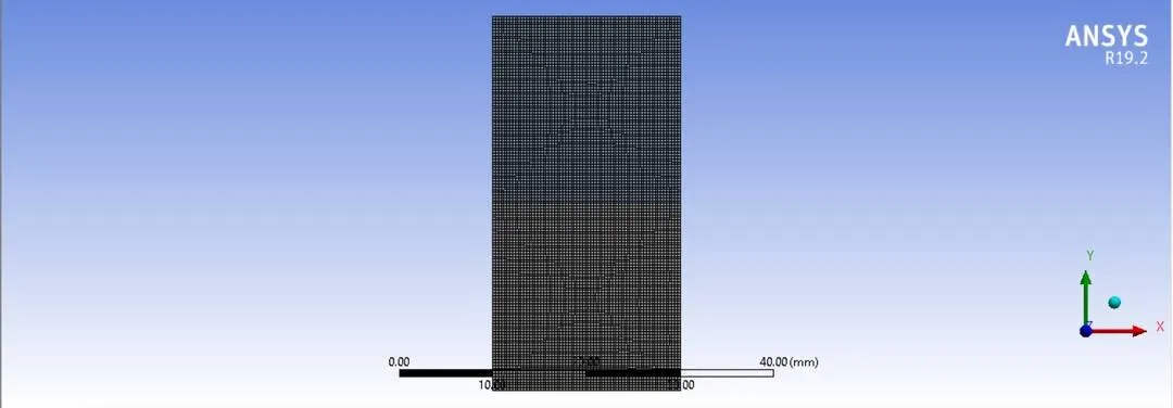
• Case 2. Mesh details: Mesh -0.3mm Element size, Elements –8978, Nodes –9180.
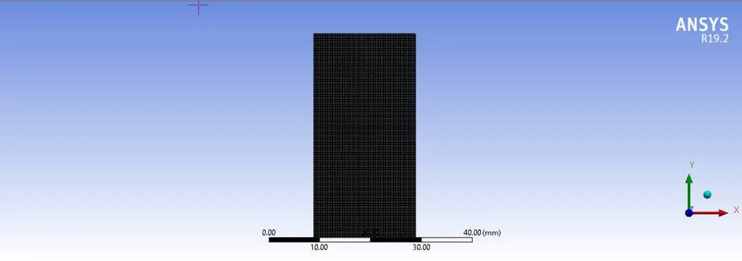
• Case 3. Mesh details: Mesh -0.2 mm Element size, Elements –20000, Nodes –20301
• Case 4(user defined material).Mesh details: Mesh -0.2 mm Element size, Elements –20000,Nodes–20301.

case setup:

• Pressure based solver and Absolute velocity is used.

• Transient-state Calculation is performed.

• Gravity is enabled in -ve Y axis

• Multiphase Model is turned on along with Volume of Fluid and number of Eulerian phases is chosen as 2 and Implicit scheme is selected.

• Viscous Model-Laminar is used.

• Cell zone selected as Fluid-air; water-surface: water-liquid.

• Patching of the volume fraction of the two phases is performed before the start of simulation. Phase used for patching was water and volume fraction of 1 is taken for water surface and 0 for air surface.

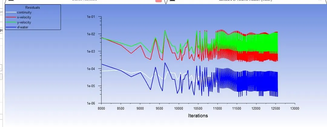
Case1:

Scaled Residuals:

Case2:

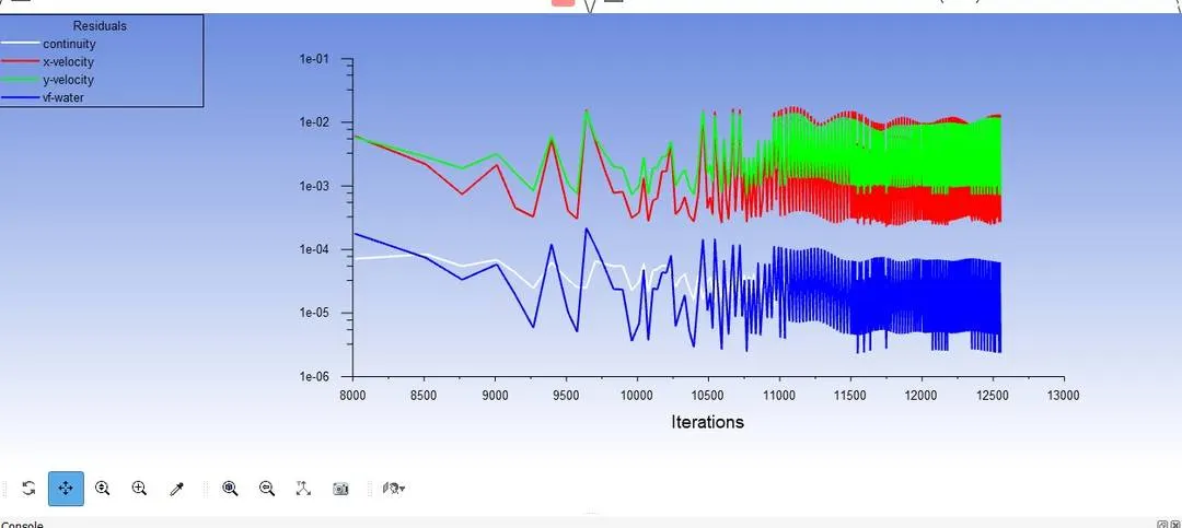
Scaled Residuals:

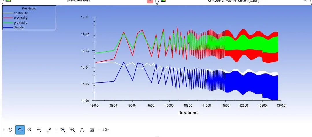
case3:

Scaled Residuals:

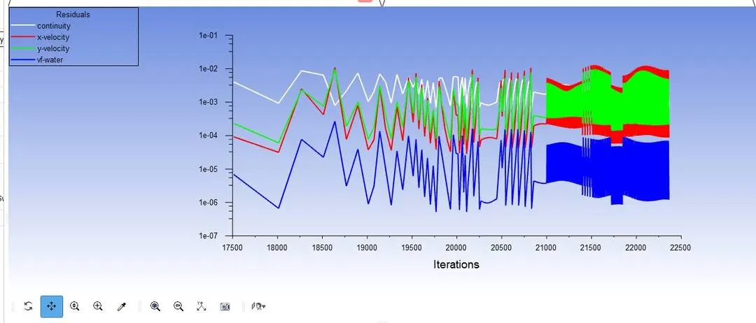
User Defined material:

Scaled Residuals:

Simulations:

https://drive.google.com/drive/folders/1CO73vepavyAbGlFE-BdSRlBJXVvelGKl?usp=sharing

Observation:

In the above cases, the simulation starts with the state of hydrostatic equilibrium and the Rayleigh Taylor instability is observed at the interference when a lower density fluid pushes a higher density fluid due to which formation of shock waves at the interface takes place. Formation of air bubbles starts taking place, which compresses the heavy fluid around it.It is observed that the more we refine the mesh, the more the simulation results get smoother about the irregularities that take place at the interface of the two fluids. As higher density fluid replaces lower density fluid, the formation of air bubbles and vortex takes place, which travels towards the upward region with time.

Steady-state approach not suitable for RT Analysis:

• The steady-state simulation is performed if we are concerned more about the final state results or the equilibrium state.
• we are more interested to study about the transition of the irregularities that starts developing when high dense fluid is upon low dense fluid under gravity effect so, by using transient solver along with refined mesh of the model, we can compute the smooth transition of irregularities that takes place at the interface of the fluids.

Atwood Number :

Atwood Number (A) is a dimensionless number which is used in study of hydrodynamic instabilities in density stratified flows. It is a dimensionless density ratio defined as

A = `(rho_1 - rho_2)/ (rho_1 + rho_2)`

`rho_1` – density of heavier fluid

`rho_2` – density of lighter fluid

It is an important parameter in study of Rayleigh Taylor instability. In Rayleigh Taylor instability the penetration of heavy fluid bubbles into the light fluid is a function of acceleration time scale `Ag t^2`.

Case 1 -3:

density of heavier fluid(water)=998.2 `(kg)/m^3`

density of lighter fluid(air)=1.225`(kg)/m^3`

Atwood Number -0.996

case4;

density of heavier fluid(water)=998.2 `(kg)/m^3`

density of lighter fluid=400 `(kg)/m^3`

Atwood Number -0.427

For Atwood number close to 0, RT instability flows take the form of symmetric fingurs of fluid.

When Atwood number close to 1, the much lighter fluid below the heavier fluid takes the form of larger bubble like plumes.