Week 6: Conjugate Heat Transfer Simulation

Aim:

• Simulate conjugate heat transfer for airflow through aluminum pipe.
• Run grid independence test on 3 grid sizes and analyze the effect of supercycle stage interval at 0.01, 0.02, and 0.03.

Theory:

Conjugate heat transfer(CHT):

The term 'conjugate heat transfer' refers to a heat transfer process involving the interaction of conduction within a solid body and the convection to the fluid moving over the solid surface. Or it is the combination of heat transfer in solids and heat transfer in fluids. The process involves temperature variations in solids and fluids, due to the thermal interaction between them. Efficiently combining heat transfer in fluids and solids is the key to designing effective coolers, heaters, or heat exchangers. CHT can be performed to improve the cooling performance of the water jacket and increase engine life.

Here we are using the supercycle method which is used for flows involving both solids and fluids because the time scale is associated with heat transfer in fluids is lesser than the time scale associated with solids. So, to converge the temperature of both solid and fluid the supercycle method is used.

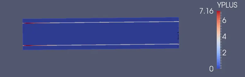
Y+ is a non-dimensional quantity and a modified form of the distance of the fluid from the wall in the boundary layer.

`Y+ = (y*ut)/v`

y = Distance of fluid from the boundary wall

ut = frictional velocity = `sqrt((tau_w)/rho)`

v = kinematic viscosity.

Calculation:

Reynolds number = 7000

The density of air @ 300k and 1atm (`rho`)= 1.1764`(kg)/m^3`

Dynamic viscosity @ 300k and 1atm (`mu`)= 1.8605e-5 `(kg)/(ms)`

Kinematic viscosity = 1.567`m^2/s`

inner pipe diameter (D) = 0.03m

Average Flow velocity = `(Re*mu)/(rho*D)` = 3.66`m/s`

Skin friction drag coefficient `c_f = 0.0576*Re^(-1/5)` = 0.0004962

wall shear stress `tau_w = 1/2*c_f*rho*v^2` = 0.0007166 `N/m^2`

Procedure:

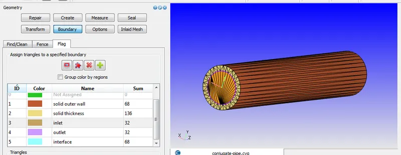
1. Geometry: Create > shape > cylinder. Do this process twice with the given dimensions which are shown in the figure below for the thickness of the cylinder.

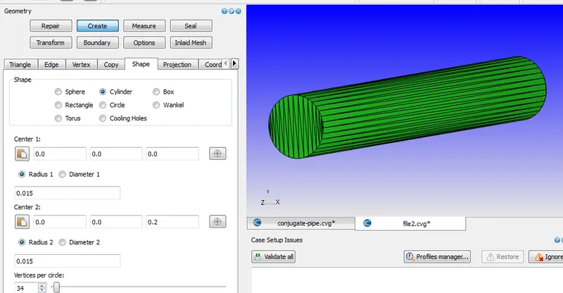
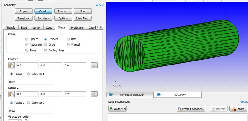
Click on diagnosis > find > then it shows the error interaction. To avoid that click > repair > delete > with by angle option select both sides of the cylinder and delete. Then click on create > triangle > loft edges > select the inner and outer circle > apply.

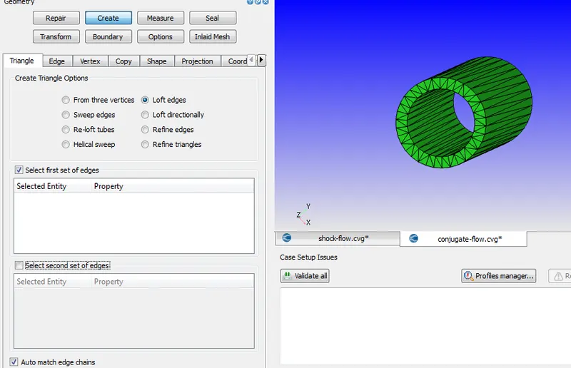
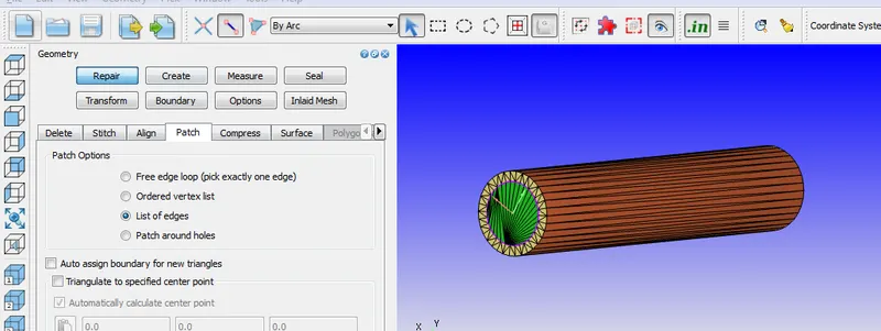
2. Now create outlet and inlet to the geometry. Repair > patch > select inner circle > apply.

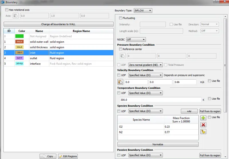
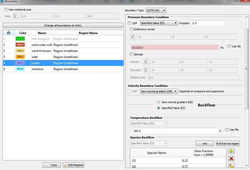
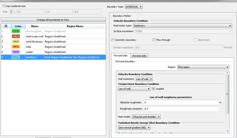
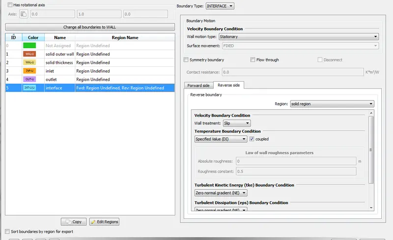
3. Set boundaries:

4. Case setup:

4.1 Application type as Time-based

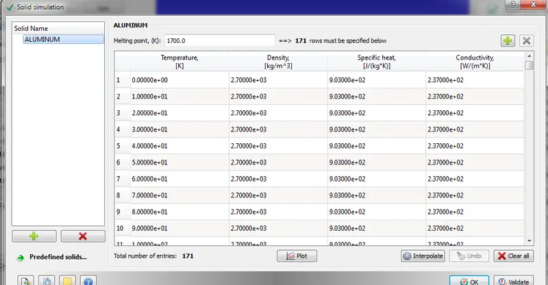
4.2 Materials: In materials select solid simulation and species.

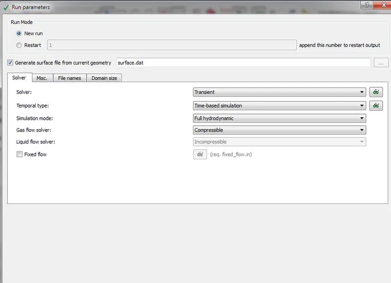
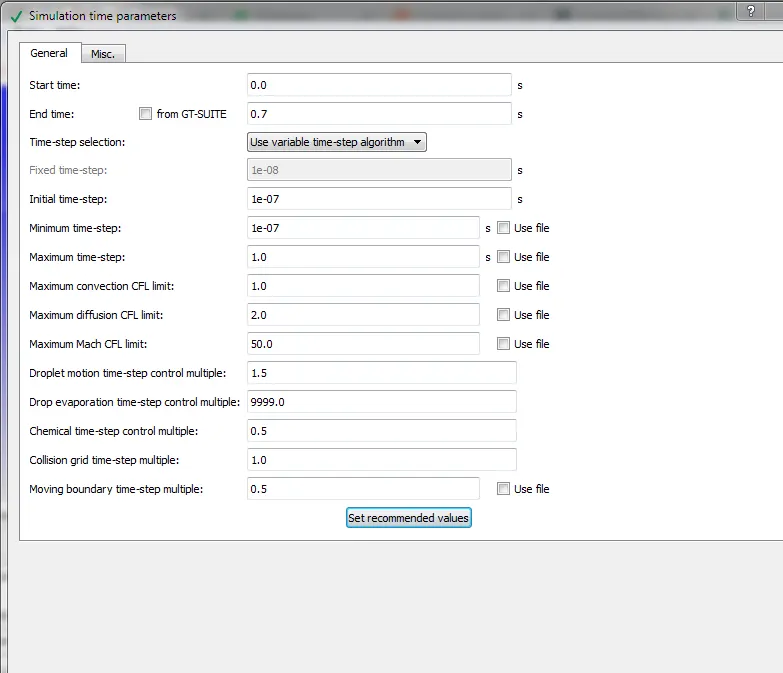
4.3 Simulation parameters: Use transient solver in the run parameters and set the time parameters.

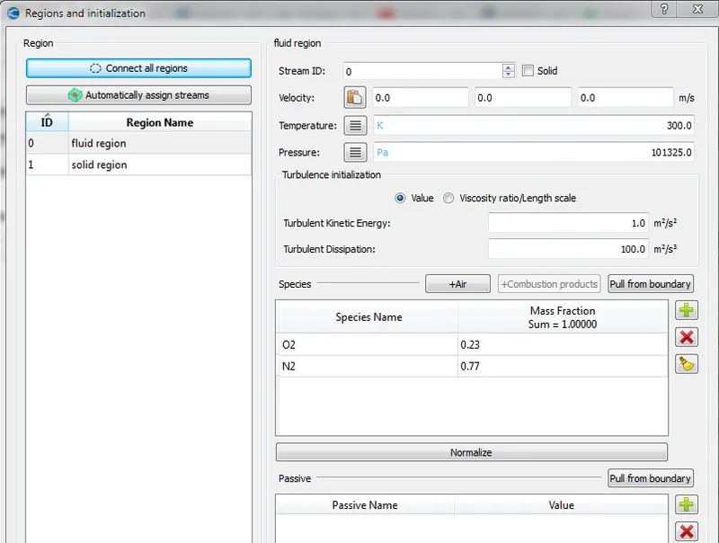
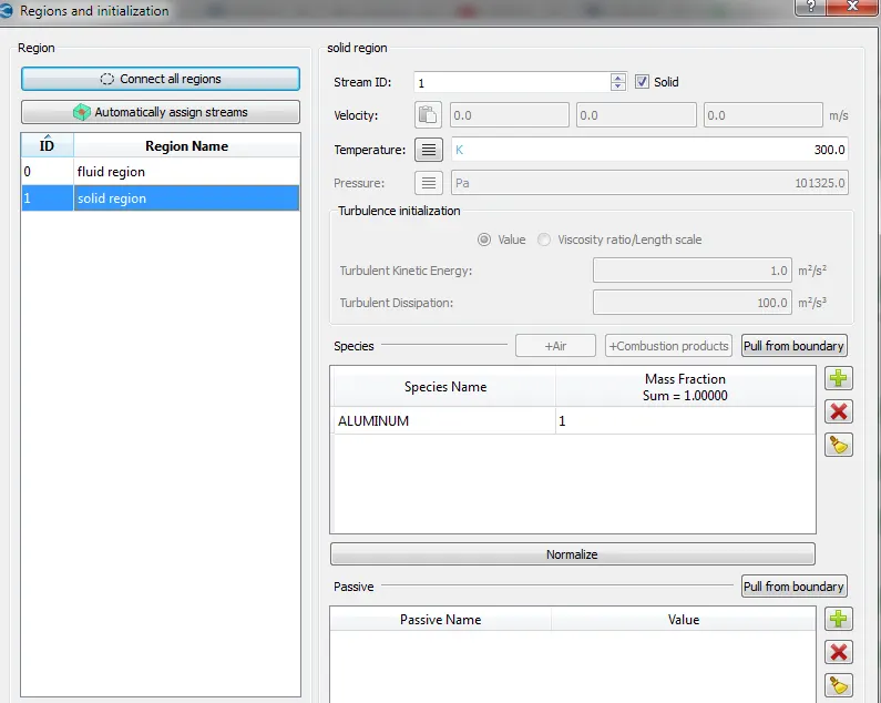
4.4 Regions and Initialization: Add 2 regions because here there is a fluid region and a solid region. Always set the fluid region as the ID 0 after that 1 for solids and ID 2 for movable solids. Create separate regions for every solid, if there are many solid regions. The stream id is very important and the region is solid then tick the solid block beside the stream ID.

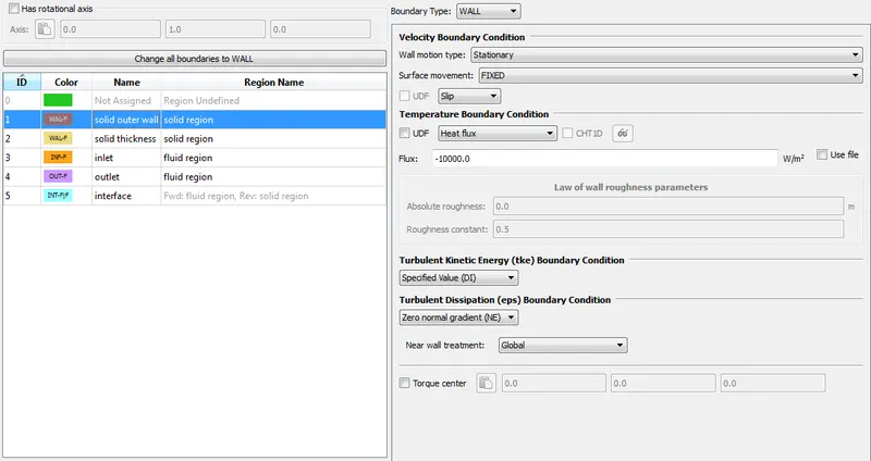
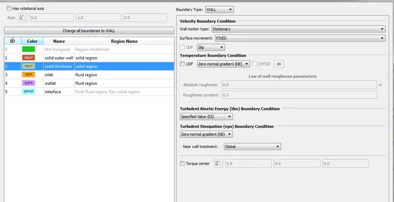
4.5 Boundary conditions:

4.6 Physical Models:

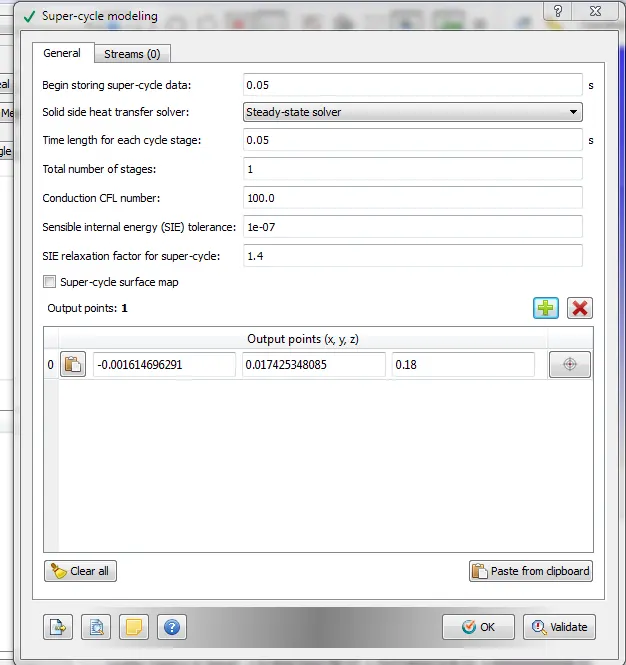
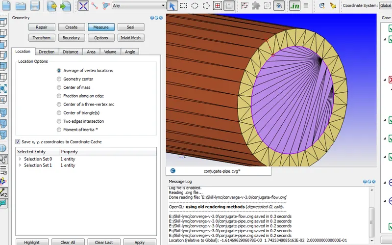
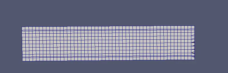
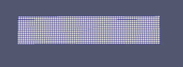
4.7 Grid control: Set mesh grid size for dx=dy=dz = 0.004.

4.8 Output/Post-processing:

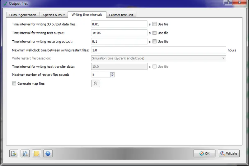
5. Now export all input files: Click on files > Export > Export input files > choose the path and select all files and press ok.

6. Run the simulation and post-convert the files: Copy and paste the mpiexec.exe file and converge.exe file to the folder in which the input files are exported to run the simulation in Cygwin. Copy the post_convert_30_msmpi_64.exe file and paste it into the output folder. Now open Cygwin and go to the output folder and type mpiexec.exe -n 4 post_convert_30_msmpi_64.exe > enter the case name(as case1) > select file type as Paraview VTK in-line binary format > type all for files and cell variables and click enter (or) we can convert those files in converge studio.

7. Post-processing the files:

To post-process the files lanch paraview and open the file location as case1 which is saved in output > case1 .. vtm (this is a group file which is formed during post-converting the files) > click on apply > create a slice along the z-axis.

Results:

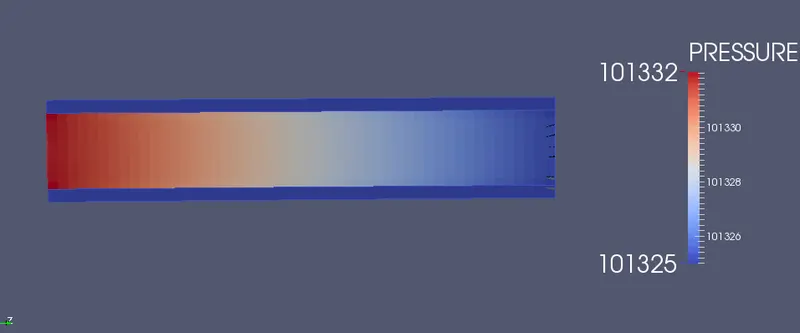
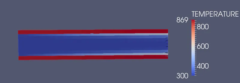
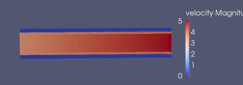
Case1: For mesh size: 0.004 The convergence temperature = 863.6 k

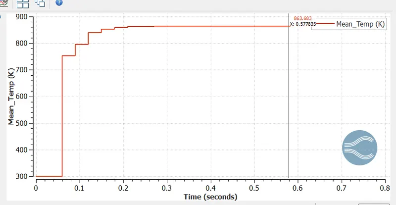
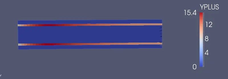
Case2: For mesh size: 0.003 The convergence temperature = 827 k

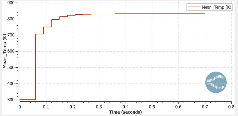
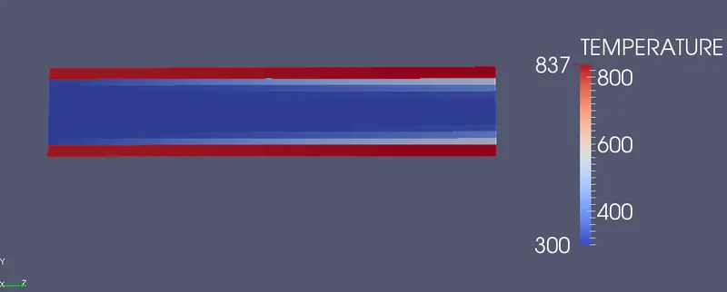
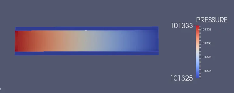
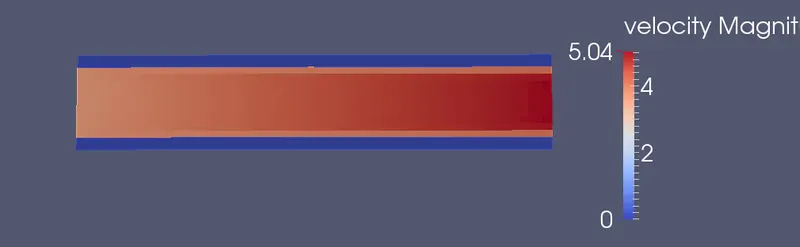
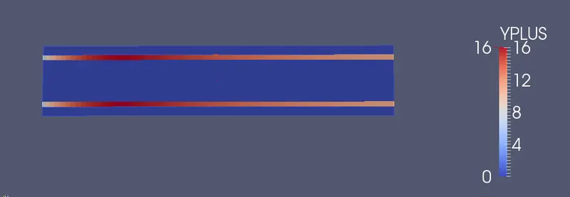
Case3: For 0.002 mesh size: The convergence temperature = 753.5 k

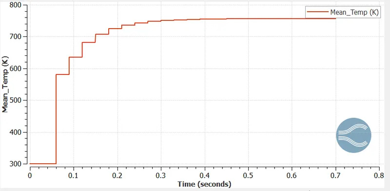
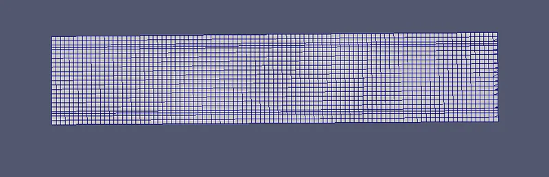
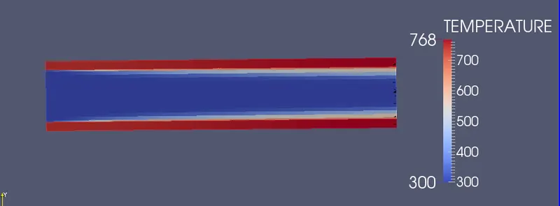
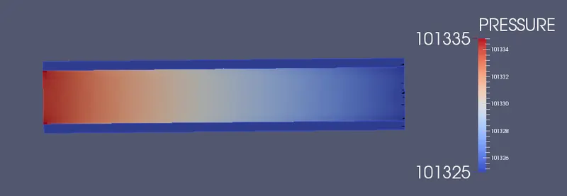
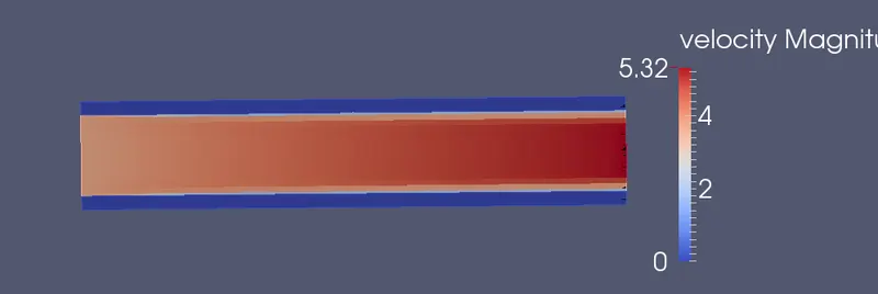
Results for 0.004 mesh size and variation in supercycle interval:

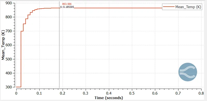
Case1: Time length for each cycle stage: 0.01

The convergence temperature remains constant because there is no change in the mesh size.

Convergence temperature = 863.56 k.

Case2: Time length for each cycle stage: 0.02

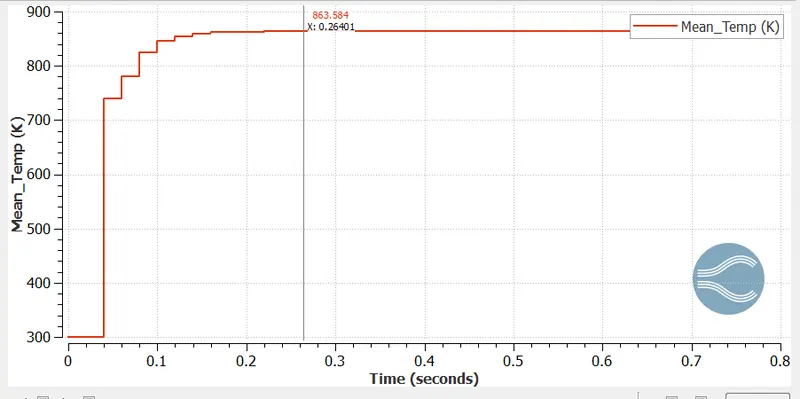
Case3: Time length for each cycle stage: 0.03

Animation link:

For mesh size 4mm: https://youtu.be/0hM1Q-yjzo0

For mesh size 3mm: https://youtu.be/bsPqo0cwL0I

For mesh size 2mm: https://youtu.be/YwHZuzIUgAA

Conclusion:

• The Y+ decreases with the mesh size, as the mesh size, decreases the flow in the viscous layer close to the wall are more accurately captured.
• The smaller the supercyclic value the convergence becomes faster and simulation time is less. For time interval 0.01 the convergence time is 0.18 sec and for 0.02 the convergence time is around 0.22 sec and for 0.03 the convergence time is around 0.29 sec. So, from the above result if we increase the supercyclic interval value the convergence time also increases. But the convergence temperature varies with the mesh size.