Genetic Algorithm

Q: Write code in MATLAB to optimise the stalagmite function and find the global maxima of the function. Plot graphs for all 3 studies and f maximum vs no. of iterations.

A: Optimisation: An optimization algorithm is a procedure which is executed iteratively by comparing various solutions until an optimum or a satisfactory solution is found.

Example: An airfoil requires a proper lift at a different angle of attack and also needs to minimise the drag. This means that the drag value should be minimum at different angles. The process of making necessary modifications in design to give minimum drag force is known as optimisation.

There are two types of algorithms. They are:

1. Deterministic algorithm: In this algorithm, specific rules are used for moving one solution to another. Output values are fully determined by input values.
2. Stochastic algorithm: These algorithms are gaining popularity due to certain properties which deterministic approach do not process.

Optimal problem formulation can be expressed by the following flow chart.

Optimisation algorithms are:

1. Single variable
2. Multiple variables
3. Constrained
4. Specialised
5. Non-traditional

Nontraditional algorithms are of two types. Genetic algorithm and Simulated algorithm.

Genetic algorithm: It is one of the optimisation processes which is a search based optimisation technique based on principles of genetic and natural selection. They are used to find optimal or near-optimal solutions. It is frequently used to solve in research and machine learning. Below flow chart represents the process of flow chart. Genetic algorithm is proposed by Charles Darwin.

Calculation of fitness function with a fitness approach can be 3 types.

1. Selection: Parents are selected from the data points.
2. Crossover: It is a process of taking two parent solutions and producing child from them
3. Mutation: It is a process carried out to maintain the genetic diversity fro one generation of a population of chromosomes to the next. If the mutation is not performed, the chromosomes will become too similar to each other, convergence takes place soon and results in local minima.

Fitness function: It takes the solution as input and produces the suitability of the solution as the output. This evaluates how close the solution is to the optimal solution of the desired problem.

Definitions:

• Variables: Parameters used in the optimisation process.
• Constraints: These are certain limits for output in the optimisation process.
• Objective function: Simple mathematical formula, which can be a predicted mathematical model that includes all variables as input.
• Variable bounds: These are the range of the input variables, that will be varied for every iteration to provide an optimised result.
• Population: To perform a genetic algorithm, the number of sample data points are required. This number is known as the population.
• Genes: These are contained in chromosomes, it is heredity transferred from parent to offspring whereas chromosomes contain hundreds of thousands of genes.

Genetic algorithm in MATLAB: In MATLAB, to find genetic algorithm, we have an in-built tool. It is used to find the minimum value of the function.

Syntax: x = ga(fun, nvars) where x is local unconstrained minimum, fun is objective function and nvars is the no.of design variables of the function.

Other syntaxes:

1. x = ga(fun, nvars, A, b)
2. x = ga(fun, nvars, A, b, Aeq, beq)
3. x = ga(fun, nvars, A, b, Aeq, beq, lb, ub)
4. x = ga(fun, nvars, A, b, Aeq, beq, lb, ub, nonlcon)
5. x = ga(fun, nvars, A, b, Aeq, beq, lb, ub, nonlcon, options)
6. x = ga(fun, nvars, A, b, [ ], [ ], lb, ub, nonlcon, IntCon)
7. x = ga(fun, nvars, A, b, [ ], [ ], lb, ub, nonlcon, IntCon, options)
8. x = ga(problem)
9. [x, fval] = ga(__)
10. [x, fval, exitflag, output] = ga(__)
11. [x, fval, exitflag, output, population, scores] = ga(__)

Where,

• A = linear inequality constraints
• b = linear inequality constraints
• Aeq = linear equality constraints
• beq = linear equality constraints
• lb = lower bounds
• ub = upper bounds
• nonlcon = non linear constarints
• options = optimisation options
• IntCon = integer variables
• x = solution
• fval = objective function value at the solution
• exitflag = reason ga stopped
• output = information about optimisation process

Note: If are any values are not given, we can represent as [ ], which means null value.

eg: x = ga(fun,nvars, [ ],[ ],[ ], [ ],lb,ub, [ ], options)

Note: Here, we calculate 3 studies for calculating a for stalagmite function. In study 1, we find with unbounded inputs, in study 2, we find by adding bounds and in study 3, we find by adding bounds and also adding population size.

Code procedure:

Stalagmite function code:

1. Add function statement for F with function name as stalagmite and input values as input.
   
   function [F] = stalagmite(input)
   
   
2. Now give input values for x and y as input(1) and input(2).
   
   x = input(1);
   
   y = input(2);
   
   
3. Write stalagmite function formulas as follows.
   
   f1 = (sin((5.1 * pi * x) + 0.5))^6;
   
   f2 = (sin((5.1 * pi * y) + 0.5))^6;
   
   f3 = exp((-4 * log(2) * ((x - 0.0667)^2)/0.64));
   
   f4 = exp((-4 * log(2) * ((y - 0.0667)^2)/0.64));
   
   F = (-1 * f1 * f2 * f3 * f4);
   
   
4. Now, end the function with end command.
   
   end
   
   
5. Save the file in the name of stalagmite_fun.

Code for stalagmite function:

function [F] = stalagmite_fun(input)

% give input values
x = input(1);
y = input(2);

% Writing stalagmite formulas
f1 = (sin((5.1 * pi * x) + 0.5))^6;
f2 = ((sin(5.1 * pi * y) + 0.5))^6;
f3 = exp((-4 * log(2) * ((x - 0.0667)^2)/0.64));
f4 = exp((-4 * log(2) * ((y - 0.0667)^2)/0.64));

F = (-1 * f1 * f2 * f3 * f4);


end

Main code:

1. Add statements as shown.
   
   clear all
   
   close all
   
   clc
   
   
2. Define search space with two variables x and y with limits 0 and 0.6.
   
   x = linspace(0, 0.6, 150);
   
   y = linspace(0, 0.6, 150);
   
   
   
3. Add value for no.of iterations that ga should perform with a variable num_cases.
   
   num_cases = 50;
   
   
4. Create 2D mesh using x and y values.
   
   [xx yy] = meshgrid(x, y);
   
   
5. Now, add tic, to know the time of the looping process.
   
   tic
   
   
6. Studying statistical behaviour with the initial values. Add loop with limit length(xx).
   
   for i = 1 : length(xx)
   
   
7. Add one more for loop with limit, length(yy).
   
   for i = 1 : length(yy)
   
   
8. Now, give values for input(1) and input(2) from 2D matrix.
   
   input(1) = xx(i, j);
   
   input(2) = yy(i, j);
   
   
9. As we have written the stalagmite function, we need to call the function and give output with a variable f.
   
   f(i, j) = stalagmite_fun(input);
   
   
10. Now, end both loops with command end.
    
    end
    
    end
    
    
11. Inputs contain row vectors containing two columns.
    
    
12. Add for loop with the size of num_cases, which is no.of iterations that need to be done in stalagmite function.
    
    for i = 1 : num_cases
    
    
13. Add ga with inputs and output variables.
    
    [inputs, fopt(i)] = ga(@stalagmite_fun, 2);
    
    
14. Adding these input values to optimum values for both x and y.
    
    xopt(i) = inputs(1);
    
    yopt(i) = inputs(2);
    
    
15. Close the for loop with end command.
    
    end
    
    
16. Now, end timing should be given to know the timing with command toc.
    
    study1_time = toc
    
    
17. Plot the 2D matrix values and objective function value with figure 1 with subplots.
    
    figure(1)
    
    subplot(2, 1, 1)
    
    hold on
    
    surfc(xx, yy, f)
    
    shading interp
    
    
18. Now, plot the optimum values with marker o, size 5, and the colour red.
    
    plot3(xopt, yopt, fopt, 'marker', 'o', 'markersize', 5, 'markerfacecolor', 'r')
    
    
19. Give title as unbounded inputs.
    
    title('unbounded inputs')
    
    
20. Plotting the optimum values of the objective function in the second subplot.
    
    subplot(2, 1, 2)
    
    plot(fopt)
    
    
21. Giving labels for X and Y-axis.
    
    xlabel('Iterations')
    
    ylabel('functions minimum')
    
    
22. Now, run the program.

Code for study 1:

clear all
close all
clc

%Defining search space
x = linspace(0, 0.6, 150);
y = linspace(0, 0.6, 150);
num_cases = 50

% creating 2D mesh
[xx yy] = meshgrid(x,y);

% study 1 - statistical behaviour
tic

 for i = 1 : length(xx)
    for j = 1 : length(yy)
        input(1) = xx(i, j);
        input(2) = yy(i, j);
        f(i, j) = stalagmite_fun(input);
    end
 end

for i = 1 : num_cases
    [inputs, fopt(i)] = ga(@stalagmite_fun, 2);   
    xopt(i) = inputs(1);
    yopt(i) = inputs(2);
end

study1_time = toc

% Plotting optimum values
figure(1)
subplot(2, 1, 1)
hold on
surfc(xx, yy, f)
shading interp
plot3(xopt, yopt, fopt, 'marker', 'o', 'markersize', 5, 'markerfacecolor', 'r')
title('unbounded inputs')
subplot(2, 1, 2)

% plotting f optimum
plot(fopt)
xlabel('Iterations')
ylabel('functions minimum')

Output for study 1: The time taken to run the loop is given as study1_time = 6.0527.

Plot for study 1:

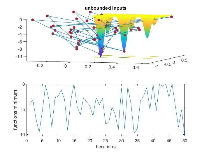
We can observe in the plot that, values are plotted all over the plot. Every time we run this, we get different values. This is because it is random sampling. In the second plot, we can observe that iteration is of 50 times and function minimum has various points.

Code procedure for study 2:

1. In this study, we are adding upper and lower bounds to reduce the points in plots in certain limits.
   
   
2. Add tic command for knowing the time taken.
   
   tic
   
   
3. Add for loop with 50 iterations.
   
   for i = 1 : num_cases
   
   
4. Add ga for stalagmite function with limits. We use [ ] when we don't have any values.
   
   [inputs, fopt(i)] = ga(@stalagmite, 2, [ ], [ ], [ ], [ ], [0 ; 0], [1 ; 1]);
   
   
5. Give optimum values as xopt and yopt.
   
   xopt(i) = inputs(1);
   
   yopt(i) = inputs(2);
   
   
6. Close the for loop with end command.
   
   end
   
   
7. Now, end timing should be given to know the timing with command toc.
   
   study2_time = toc
   
   
8. Till now we got all values and we should plot these to know ga maxima value. Add with figure(2) and subplots.
   
   figure(2)
   
   subplot(2, 1, 1)
   
   hold on
   
   surfc(xx, yy, f)
   
   shading interp
   
   
9. Now, plot the optimum values with marker o, size 5, and the colour red.
   
   plot3(xopt, yopt, fopt, 'marker', 'o', 'markersize', 5, 'markerfacecolor', 'r')
   
   
10. Give title as unbounded inputs.
    
    title('bounded inputs')
    
    
11. Plotting the optimum values of the objective function in the second subplot.
    
    subplot(2, 1, 2)
    
    plot(fopt)
    
    
12. Giving labels for X and Y-axis.
    
    xlabel('Iterations')
    
    ylabel('functions minimum')
    
    
13. Now, run the program.

Code for study 2:

% study 2 - statistical behaviuor - with upper and lower bounds
tic
for i = 1 : num_cases
    [inputs, fopt(i)] = ga(@stalagmite_fun, 2, [], [], [], [], [0 ; 0], [1 ; 1]);   
    xopt(i) = inputs(1);
    yopt(i) = inputs(2);
end
study2_time = toc

% Plotting optimum values
figure(2)
subplot(2, 1, 1)
hold on
surfc(xx, yy, f)
shading interp
plot3(xopt, yopt, fopt, 'marker', 'o', 'markersize', 5, 'markerfacecolor', 'r')
title('bounded inputs')
subplot(2, 1, 2)

% plotting f optimum
plot(fopt)
xlabel('Iterations')
ylabel('functions minimum')

Output for study 2: The time taken to run the loop is given as study2_time = 6.6568.

Plot for study 2:

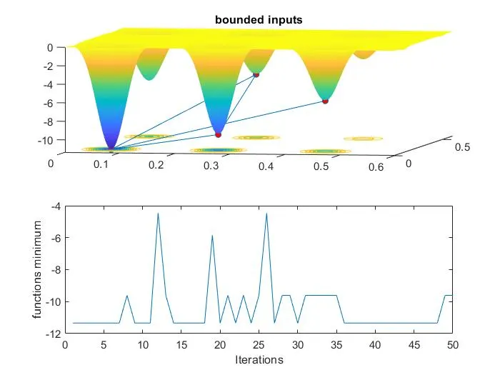
We get a plot little clear. We observe that the function predicts the minimum point is between peaks(not everywhere). The range is also decreased. By reducing search space, we get a more clear plot of minima value.

Code procedure for study 3:

1. In this study, we are reducing the upper and lower bounds to reduce the points in plots in certain limits. We know ga performs with random samples. By default, ga takes 50 samples. We are increasing the population size because fro lower population size, it is difficult to find the value. We can find the local value. Increasing the population size can slow down the ga because we have more samples, more individuals and processing etc.
   
   
2. Add value for options command as follows.
   
   options = optimoptions('ga');
   
   
3. Add population size as 600.
   
   options = optimoptions(options, 'PopulationSize', 400);
   
   
4. Add tic command for knowing the time taken.
   
   tic
   
   
5. Add for loop with 50 iterations.
   
   for i = 1 : num_cases
   
   
6. Add ga for stalagmite function with limits. We use [ ] when we don't have any values. Decreasing the lower and upper bounds.
   
   [inputs, fopt(i)] = ga(@stalagmite, 2, [ ], [ ], [ ], [ ], [0 ; 0], [0.1 ; 0.1], [ ], [ ], options);
   
   
7. Give optimum values as xopt and yopt.
   
   xopt(i) = inputs(1);
   
   yopt(i) = inputs(2);
   
   
8. Close the for loop with end command.
   
   end
   
   
9. Now, end timing should be given to know the timing with command toc.
   
   study3_time = toc
   
   
10. Till now we got all values and we should plot these to know ga maxima value. Add with figure(3) and subplots.
    
    figure(3)
    
    subplot(2,1,1)
    
    hold on
    
    surfc(xx, yy, f)
    
    shading interp
    
    
11. Now, plot the optimum values with marker o, size 5, and the colour red.
    
    plot3(xopt, yopt, fopt, 'marker', 'o', 'markersize', 5, 'markerfacecolor', 'r')
    
    
12. Give title as unbounded inputs.
    
    title('bounded inputs with population size')
    
    
13. Plotting the optimum values of the objective function in the second subplot.
    
    subplot(2,1,2)
    
    plot(fopt)
    
    
14. Giving labels for X and Y-axis.
    
    xlabel('Iterations')
    
    ylabel('functions minimum')
    
    
15. Now, run the program.

Code for study 3:

%Study 3 increasing GA iteration
options = optimoptions('ga');
options = optimoptions (options, 'PopulationSize', 400);

tic
for i = 1 : num_cases 
    [inputs, fopt(i)] =  ga(@stalagmite_fun, 2, [], [], [], [], [0;0],[0.1;0.1], [],[],options);   
    xopt(i) = inputs(1);
    yopt(i) = inputs(2);
end

study3_time = toc

% Plotting optimum values
figure(3)
subplot(2, 1, 1)
hold on
surfc(xx, yy, f)
shading interp
plot3(xopt, yopt, fopt, 'marker', 'o', 'markersize', 5, 'markerfacecolor', 'r')
title('bounded inputs with population size')
subplot(2, 1, 2)

% plotting f optimum
plot(fopt)
xlabel('Iterations')
ylabel('functions minimum')

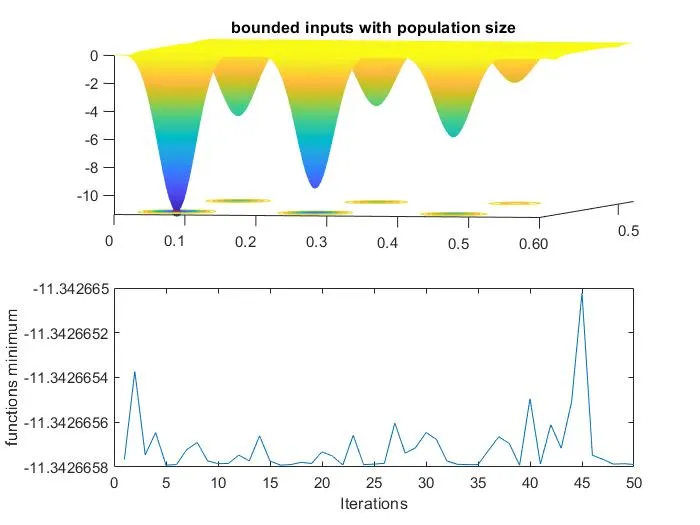
Output for study 3: The time taken to run the loop is given as study3_time = 43.1270.

Plot for study 3: We can observe that only one point is visible in the plot at the peak point. This is the maximum value for stalagmite function. This is achieved by increasing the population size and giving necessary limits for the function.

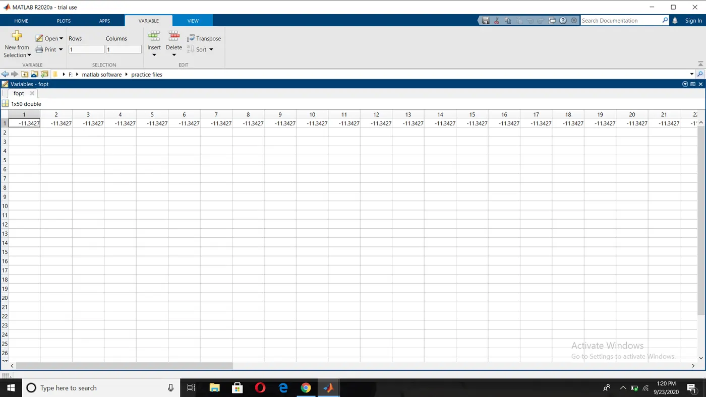
Final values in the workspace:

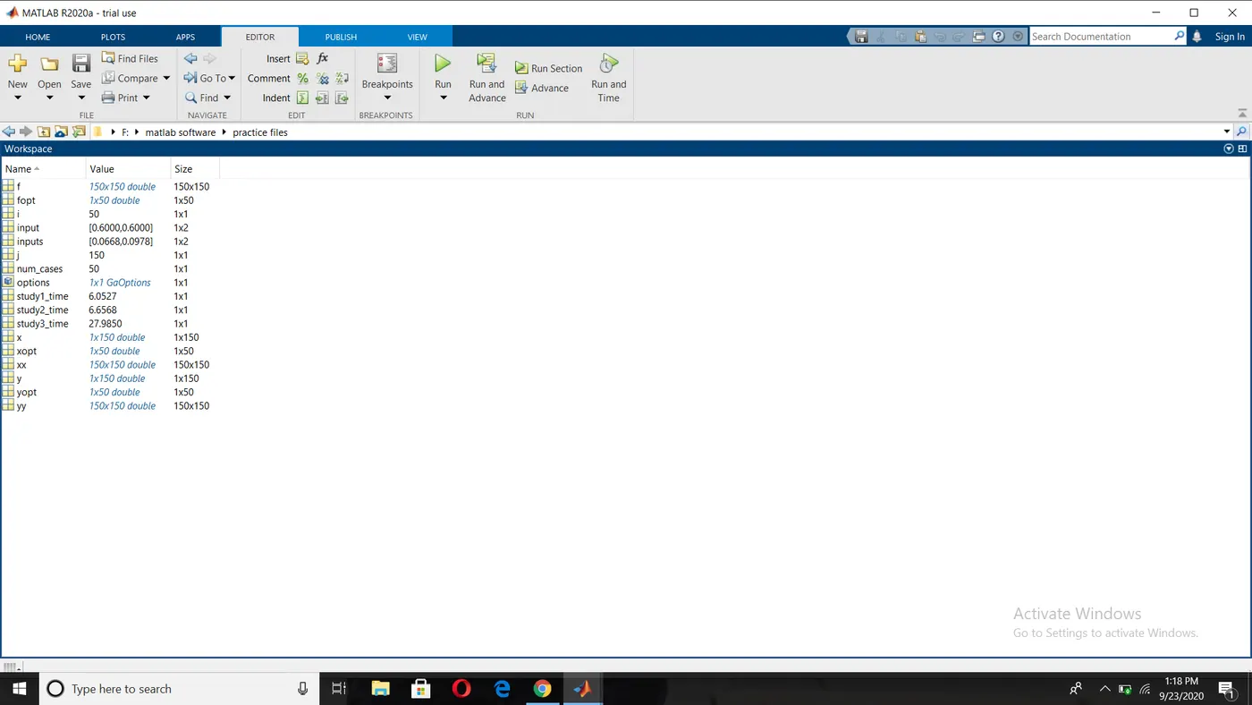
Final fopt values:

Points to remember:

• Write values in syntaxes accordingly, without any errors.
  
  
• Write all three studies in a single script and run the program individually. This can be done by selecting the each study and right click on it. A box appears and select 'Evaluate selection'. This can also be done by pressing F9 after selecting each study code.
  
  
• If there are no values present in syntax, give [ ] for them.
  
  
• plot3 is a command where the point can be denoted in the 3D figure.
  
  
• Stalagmite function formulas should be written carefully.
  
  
• tic and toc command should be used for starting and ending of the for loops.
  
  
• Subplot command is used for plotting more plots in a single plot. Syntax is subplot(m,n,p). where m and n are no.of rows and columns and p is a position of plot in a figure.

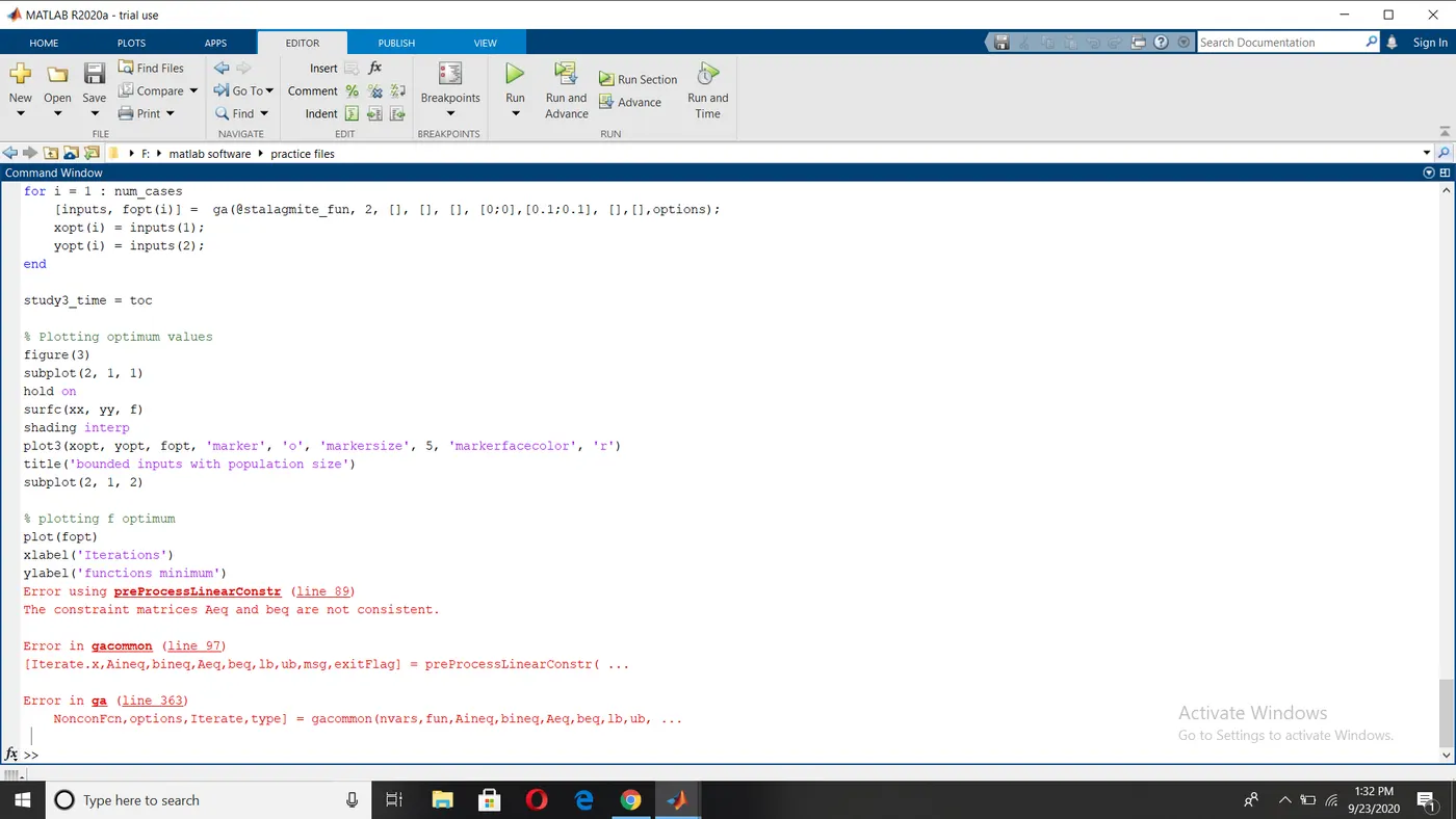
Errors and their rectification:

1. Below is the error when you give inputs insufficiently in syntax. This can be solved by checking syntax and writing correctly.
   

References:

https://skill-lync.com/knowledgebase/genetic-algorithm-explained

https://mech.iitm.ac.in/nspch52.pdf

https://www.mathworks.com/help/gads/ga.html

Conclusion:

Therefore, optimum values have been calculated for three studies and plotted each. Global maxima of stalagmite function is calculated.