Solving second order ODEs - Simple Pendulum

The aim of the soulution is to get a result of positions of the pendulum and the velocities at the obtained positions, by soliving the ODE for the simple pendulum.

The ODE for the simple pendulum is given by :

`[d^2(theta)]/dt+(b/m)(d(theta))/(dt)+(g/l)sin(theta)=0`

To solve the second order ODE, we convert it into a first order ODE and then use the matlab functions and solvers to solve the ODE.

The solution is in the form of a matrix that gives the position and the velocity as a function of time.

The following is the code and the function used :

clear all 
close all
clc
%program to solve ODE for pendulum motion

g= 9.81;
l= 1;
m=1;
b=0.05;

%initial conditions
theta_0= [0; 3];
tspan= linspace(0,20,100);

%ODE solution
[t, results] = ode45(@(t,theta) ode_func(t,theta,b,g,l,m),tspan,theta_0);

plot( t, results(:,1))
hold on
plot(t,results(:,2))
ylabel('position and velocity')
xlabel('time')

%Making a Movie
%obtaining angular positions of the pendulum
z=results(:,1);
frame=1;

for i=1:length(z)
    x=l*sin(z(i));
    y=-l*cos(z(i));
    figure(2)
    plot([0,x],[0,y],'linewidth',2)
    hold on
    plot(x,y,'o','MarkerSize',20)
    hold off
    axis([-1 1 -1.5 0.5])
    %frames for the position
    M(frame)=getframe(gcf);
    frame=frame+1;
    
end
%making an animation
movie(M)
videofile = VideoWriter('Simple_Pendulum_animation.avi','Uncompressed AVI');
open(videofile)
writeVideo(videofile,M)
close(videofile) 
    

Function code:

function [dtheta_dt] = ode_func(t,theta,b,g,l,m)
theta1 = theta(1);
theta2=theta(2);
dtheta1_dt = theta2;
dtheta2_dt = -(b/m)*theta2 - (g/l)*sin(theta1);
dtheta_dt=[dtheta1_dt; dtheta2_dt];
end

theta1 represents position and the derivative of theta1 which is theta 2 gives the velocity, both as a function of time. In the main code, the above function is used in ode45 solver, which finally gives the value of time and theta. As theta has two variables in it i.e, position and velocity, the result is a two column matrix with number of rows depending on the time intervals the ode is solved at.

For our case, the time is divided into 100 parts between 0 and 20 secs using linspace(0,20,100) command. The intital conditions for the ODE are theta_0 with position at 0 and velocity at 3 rads/ sec. The solver solves the equation and outputs results with first column as position in rads and second column as velocity in rads/sec.

The plot is as follows:

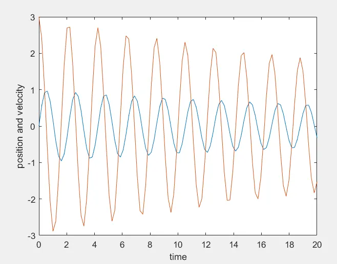
As the damping value b=0.05 is very less, we see oscillations continuing without much damping.

The blue line represents the position and the red line represents the velocity.

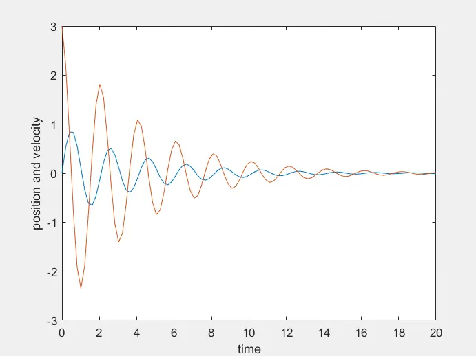
Increasing b value to 0.5 damps the oscillations quicker as shown in the figure below.

To obtain the animation of the movement of the pendulum, we plot:

• One end of the pendulum which is fixed at origin (0,0).
• The other end moves according to the solution of the ODE we solved.

If the instanataneous co ordinate of pendulum is taken as (x,y) then

`x=lsin(theta)`

`y=-lcos(theta)` // as the pendulum moves in negative y axis

l is the length of the pendulum.

We iterate the position of the pendulum using for loop by taking the values from the results as z and plotting the graph for every positional value from 1 to 100 rows. As there are 100 values for the positions, there will be 100 iteratons and each iteration is saved as a frame to make a movie of them later.

The pendulum in the animation is represented by the spherical marker. The axis limits are taken from -1 to 1 for x axis and -1.5 to 0.5 for y axis for visual purpose.

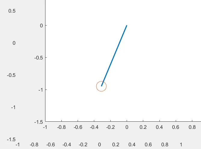
The above figure shows the frame for a particular period of time with a particular position.

The animation can be seen by opening the appropriate link provided below.

Code links:

https://drive.google.com/file/d/15mOQ_qdkJe_lIfNQ9TToKZZ546G75QB0/view?usp=sharing

https://drive.google.com/file/d/1OV2mEPtJnmd8sQwoJReSh0EGrjEbwAW7/view?usp=sharing

Animation link:

https://drive.google.com/file/d/1j4mUJAnNRWIE_YBT1QVvynIBoTVOVrXy/view?usp=sharing