Week 3 - Solving second order ODEs

Object:

Your objective is to write a program that solves the following ODE. This ODE represents the equation of motion of a simple pendulum with damping

Code:

clear all
close all 
clc

b=0.05;
g=9.81;
l=1; %length is m
m=1; %mass is kg
%Initial condition
theta_0=[0;3];

%time point
t_span=linspace(0,20,150);

%Slove ODE
[t,result]=ode45(@(t,theta)ode_function(t,theta,b,g,l,m),t_span,theta_0);

plot(t,result(:,1))
hold on 
plot(t,result(:,2))
xlabel('time')
ylabel('angular displacement')

%Animation
X0=0;
Y0=0;

ct=1;
for i=1:length(t)
    X1=l*sin(result(i,1));
    Y1=-l*cos(result(i,1));

    figure(2)
    plot([-1 1],[0 0],'LineWidth',6,'Color','g');
    axis([-2 2 -2 2]);
    line([X0 X1],[Y0 Y1],'linewidth',4,'color','b');
    hold on;
    plot(X0,Y0,'O','MarkerSize',3,'MarkerFaceColor','y');
    plot(X1,Y1,'O','MarkerSize',20,'MarkerFaceColor','r');
    title('Damping of simple pendulum');
    grid on;
    hold off;
    M(ct)=getframe(gcf);
    ct=ct+1;
end

movie(M);
videofile=VideoWriter('simple_pendulum.avi','Uncompressed AVI');
open(videofile);
writeVideo(videofile,M);
close(videofile);

Function code:

function [dtheta_dt] = ode_function(t,theta,b,g,l,m)
    theta1 = theta(1)
    theta2 = theta(2)
    dtheta1_dt = theta2;
    dtheta2_dt = -(b/m)*theta2 - (g/l)*sin(theta1);
    dtheta_dt = [dtheta1_dt; dtheta2_dt];
end

output:

figure:1

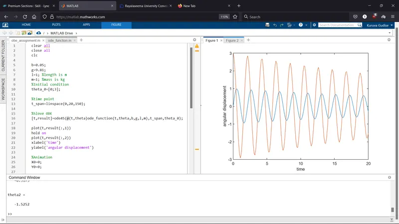
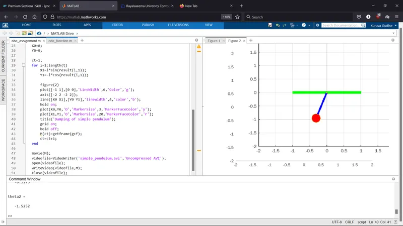
figure:2

youtube link: https://youtu.be/-WqDj_m9Iog

Report:

Solving the second order ODE to find the oscillation of simple pendulum.

Using terms:

b-damping ratio

m-mass

g-gravity

l-length

The length of bob is 1m, mass of bob is 1kg, gravity is 9.81 and damping ratio is 0.05

Theta_0 as contain the displacement and velocity is [ 0; 3]

Timespan is taken linspace 0 to 20 it as divided in 150 times.

%Solve ODE

Ode45 is the inbuilt function of solved in Matlab and ODE45 is usually the function of choice among the ODE solvers. it compares methods of orders four and five to estimate error and determine the step size. ODE45 is so accurate that its default behavior is to use its interpolant to provide result at intermediate point.

It as represents in [t, result] equal to ode45 off main function, ode function definition, time array and initial conditions

[t, result] = ode45(@ (t, theta)ode_function(t, theta, b, g, l, m), t_span, theta_0)

Function

Function is nothing but a piece of code that we can reuse by just calling its name and passing in right parameters.

This is the Function code

function [dtheta_dt] = ode_function(t, theta, b, g, l, m)

theta1 = theta (1)

theta2 = theta (2)

dtheta1_dt = theta2;

dtheta2_dt = -(b/m) *theta2 - (g/l) *sin(theta1);

dtheta_dt = [dtheta1_dt; dtheta2_dt];

End

Plotting:

Plot the points in time and results of first column hold on and plot the points of second column.

Xlabel is time and ylabel is angular displacement.

%ANIMATION

Starting point of pendulum is X0, Y0.

Use ct=1

Counter actually represents the each and every frame

For loop

For statements loop a specific number of times and keep track of each iteration with an incrementing index variable.

Using for loop I should be taken as 1 to length of t

X1=length*sin(result(I,1)) and y1=-l*cos(result(I,1))

Plot the horizontal line x-axis from –1 to 1, length of support is 6 in color of green and the axis range of x-axis is –2 to 2 and y-axis is –2 to 2.

Line as represent the length of connecting rod starting point [X0 X1], [Y0 Y1] and the length is 4 in color of blue

Plot the point of X0, Y0 In represent of circle, markersize of 3 and markerfacecolor in yellow

Plot the point of X1, Y1 In represent of circle, markersize of 20 and markerfacecolor in red

The title is Damping of simple pendulum and grid on

Creating the plot animation to use M(CT)= getframe(gcf), ct=ct+1 and the commands used is

movie(M)

videofile=VideoWriter('simple_pendulum.avi','Uncompressed AVI')

open(videofile)

writeVideo(videofile,M)

close(videofile)

the file should be saved as Simple_pendulum.avi is as saved in video format.

when i run the program i didn't face any errors in command window