Week 3 - Solving second order ODEs
Aim : solving second order ode using matlab.
Objective: write a program that solves the following ODE. This ODE represents the equation of motion of a simple pendulum with damping.
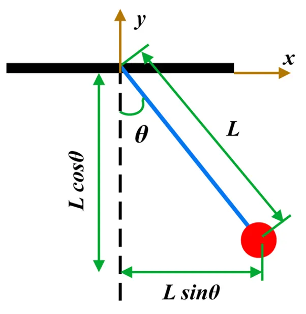
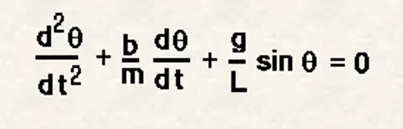
In the above equation,
g = gravity in m/s2,
L = length of the pendulum in m,
m = mass of the ball in kg,
b=damping coefficient.
Function definition:
% function code
%using x instead of theta and x dot is an output variable of function
function xdot=main_func_ode(t,x)
% given values and consider this values as constant.it is same for mass(m),g and length(l)
b = 0.05;
g = 9.81;
l = 1;
m = 1;
%assigning null matrix to xdot
xdot =zeros(2,1);
% first element is angular velocity,which is at x(2) position
xdot(1)=x(2);
% this will obtain after conversion of 2nd order ode to 1st order ode
xdot(2) = -(b/m)*(2)-(g/l)*sin(x(1));
end
main program:
clear all;
close all;
clc;
%inputs
l=1;
t=linspace(0,20,100);
x0 =[0 3];
Syntax ode45:
[t,y] = ode45(odefun,tspan,y0)
[t,y] = ode45(odefun,tspan,y0,options)
[t,y,te,ye,ie] = ode45(odefun,tspan,y0,options)
Description:
[t,y] = ode45(odefun,tspan,y0), where tspan = [t0 tf], integrates the system of differential equations y′=f(t,y) from t0 to tf with initial conditions y0. Each row in the solution array y corresponds to a value returned in column vector t.
All MATLAB® ODE solvers can solve systems of equations of the form y′=f(t,y), or problems that involve a mass matrix, M(t,y)y′=f(t,y). The solvers all use similar syntaxes. The ode23s solver only can solve problems with a mass matrix if the mass matrix is constant. ode15s and ode23t can solve problems with a mass matrix that is singular, known as differential-algebraic equations (DAEs). Specify the mass matrix using the Mass option of odeset.
ode45 is a versatile ODE solver and is the first solver you should try for most problems. However, if the problem is stiff or requires high accuracy, then there are other ODE solvers that might be better suited to the problem. See Choose an ODE Solver for more information.
[t,y] = ode45(odefun,tspan,y0,options) also uses the integration settings defined by options, which is an argument created using the odeset function. For example, use the AbsTol and RelTol options to specify absolute and relative error tolerances, or the Mass option to provide a mass matrix.
[t,y,te,ye,ie] = ode45(odefun,tspan,y0,options) additionally finds where functions of (t,y), called event functions, are zero. In the output, te is the time of the event, ye is the solution at the time of the event, and ie is the index of the triggered event.
Examples:
ODE with Single Solution Component
Simple ODEs that have a single solution component can be specified as an anonymous function in the call to the solver. The anonymous function must accept two inputs (t,y), even if one of the inputs is not used in the function.
Solve the ODE
y′=2t.
Specify a time interval of [0 5] and the initial condition y0 = 0.
tspan = [0 5];y0 = 0;[t,y] = ode45(@(t,y) 2*t, tspan, y0);
% solving differential equation using ode45 %(matlab inbuild function)
[t,x]=ode45('main_func_ode',t,x0);
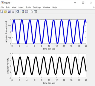
% plotting for tracing of angular velocity and angular displacement
subplot(2,1,1)
plot(t,x(:,1),'-b','linewidth',4);
xlabel('time t in sec');
ylabel('angular displacement');
subplot(2,1,2);
hold on;
plot(t,x(:,2),'-k','linewidth',4);
xlabel('time t in sec');
ylabel('angular velocity');
grid on;
Error:
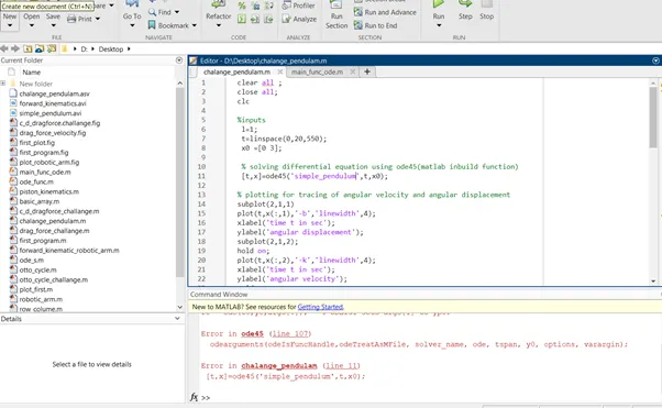
While running the program there is the error shown in fig ,Actually they need to same in function name and file name.after entering both names same ,the program is running good, and show the results well.
% animation
X0 =0;
Y0 =0;
ct=1; % counter actually represents each and every frame
for loop:
A for loop is a repetition control structure that allows you to efficiently write a loop that needs to execute a specific number of times.
values can be one of the following forms: initval:endval --- increments the index variable from initval to endval by 1, and repeats execution of program statements until index is greater than endval. Initval:step:endval --- increments index by the value step on each iteration, or decrements when step is negative. valArray --- creates a column vector index from subsequent columns of array valArray on each iteration. For example, on the first iteration, index = valArray(:,1). The loop executes for a maximum of n times, where n is the
number of columns of valArray, given by numel(valArray, 1, :). The input valArray can be of any MATLAB data type, including a string, cell array, or struct.
Example
for a = 10:20
fprintf('value of a: %d\n', a);
end
When the code above is executed, the result will be:
value of a: 10
value of a: 11
value of a: 12
value of a: 13
value of a: 14
value of a: 15
value of a: 16
value of a: 17
value of a: 18
value of a: 19
value of a: 20
while we are using for loop function we can get the animation for our simple pendulum using 2nd order .
for i= l:length(t)
X1=l*sin(x(i,1))
Y1=l*cos(x(i,2));
figure(2)
plot([-1 1],[0 0],'Linewidth',6,'Color','r');
axis([-2 2 -2 2]);
line([X0 X1],[Y0 Y1],'Linewidth',2,'Color','b');
hold on
plot(X0,Y0,'O','markersize',3,'markerfacecolor','y');
plot(X1,Y1,'O','markersize',20,'markerfacecolor','r');
title('damping of simple pendulum');
legend('support rod','length of pendulum','fix point','Ball of pendulum');
grid on
hold off;
M(ct) = getframe(gcf);
ct = ct+1 ;
end
movie(M);
videofile = VideoWriter('simple_pendulum','Uncompressed AVI');
open(videofile);
writeVideo(videofile,M);
close(videofile);
commands used in this program:
clc: Clears command window.
clear :Removes variables from memory.
Close :Closes all plots.
Length :Computes number of elements.
Linspace :Creates regularly spaced vector.
Axis :Sets axis limits.
Grid :Displays gridlines.
Plot : Generates xy plot.
Figure : Opens a new figure window.
Xlabel : Adds text label to x-axis.
ylabel : Adds text label to y-axis.
Hold : Freezes current plot.
click on the below link to see the animation of simple pendulum.
https://drive.google.com/file/d/1WVi62jHRpYKCqC2PiF8pNgVcfRvCA4WX/view?usp=sharing
conclusion:
finally we got an animation of simple pendulum using the matlab
% function code
function xdot=main_func_ode(t,x) %using x instead of theta and x dot is an output variable of function
     b = 0.05; % given values and consider this values as constant.it is same for mass(m),g and length(l)
     g = 9.81;
     l = 1;
     m = 1;
     xdot =zeros(2,1); %assigning null matrix to xdot
     xdot(1)=x(2); % first element is angular velocity,which is at x(2) position
     xdot(2) = -(b/m)*(2)-(g/l)*sin(x(1)); % this will obtain after conversion of 2nd order ode to 1st order ode
end

%main code

clear all ;
close all;
clc

%inputs
 l=1;
 t=linspace(0,20,100);
 x0 =[0 3];

 % solving differential equation using ode45(matlab inbuild function)
 [t,x]=ode45('main_func_ode',t,x0);

% plotting for tracing of angular velocity and angular displacement
subplot(2,1,1)
plot(t,x(:,1),'-b','linewidth',4);
xlabel('time t in sec');
ylabel('angular displacement');
subplot(2,1,2);
hold on;
plot(t,x(:,2),'-k','linewidth',4);
xlabel('time t in sec');
ylabel('angular velocity');
grid on;
% animation


ct=1; % counter actually represents each and every frame

for i= l:length(t)
    X0 =0;
    Y0 =0;
    X1=l*sin(x(i,1));
    Y1=l*cos(x(i,2));


    figure(2)
    plot([-1 1],[0 0],'Linewidth',6,'Color','r');
    axis([-2 2 -2 2]);
    line([X0 X1],[Y0 Y1],'Linewidth',2,'Color','b');
    hold on
    plot(X0,Y0,'O','markersize',3,'markerfacecolor','y');
    plot(X1,Y1,'O','markersize',20,'markerfacecolor','r');
    title('damping of simple pendulum');
    legend('support rod','length of pendulum','fix point','Ball of pendulum');
    grid on
    hold off;
    M(ct) = getframe(gcf);
    ct = ct+1 ;

end
movie(M);
videofile = VideoWriter('simple_pendulum','Uncompressed AVI');
open(videofile);
writeVideo(videofile,M);
close(videofile);
https://drive.google.com/file/d/1WVi62jHRpYKCqC2PiF8pNgVcfRvCA4WX/view?usp=sharing