Week 3: Flow over a backward facing step
Aim:
To set up the backward-facing step case in converge environment and post-process the result in the Paraview
Introduction:
The flow is through the backward-facing step. In this project converge studio is used to set up the profile, the solver settings, and the initial conditions. The flow is driven by the change in the pressure difference between the inlet and the outlet.
Procedure:
Geometry:
The geometry is downloaded from the given data. Checking the orientation of the Normals which have to be inward to the geometry. Running the diagnosis to check any open edges or faces.
Boundary Flagging:
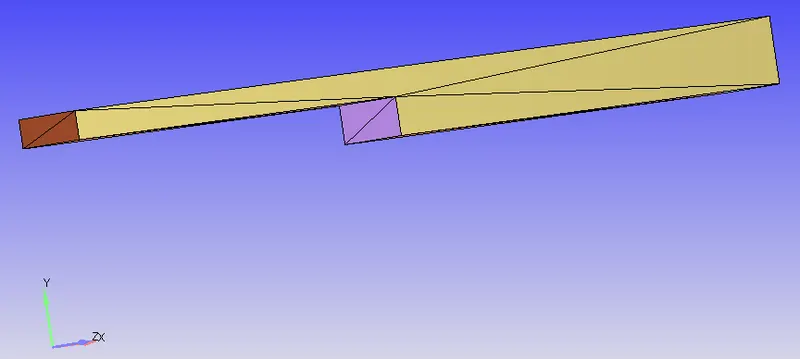
The boundaries are flagged using triangular blocks on the geometry.
Inlet, Outlet, Top and Bottom walls, Front 2D and Back 2D boundaries are created and selected respective sections.
Case Setup:
Application: Time Based
Materials: Air
Reaction mechanism: YES
Species: YES
Species: O2 & N2
Run Parameters:
Solver: Steady-state Solver
Misc: Steady-State monitor and no Shared memory
Simulation time: End Time: 15000
Initial Time Step: 1e-6
Minimum Time step: 1e-6
Max Convection CFL: 1
Solver Parameters: Density Based
Equations: Solver: Converge Bicgstab
Preconditioner: None
Steady-State solver Control: Maximum CFL limit: 0.5
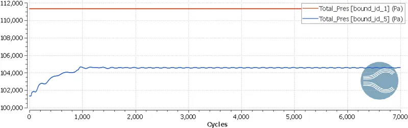
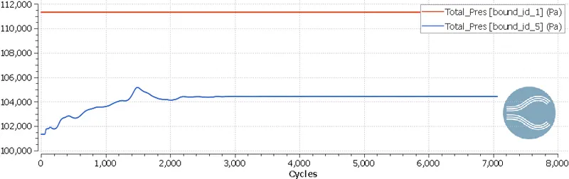
Boundary: Inlet: Inflow > Pressure boundary condition 111325 > Temperature Boundary conditions 300K > Species air
Outlet: Outflow > Pressure 101325 > Temperature 300 > Species air
Top_Bottom: Walls > Law of wall
Front & Back:2D condition
Regions: species interchange the fraction of N2 and O2 and Name the region as the volumetric region
Physical Model: Turbulence model RNG k-`varepsilon` model Grid: Grid_1: 2e-4 2e-4 2e-4
Grid_2: 1.5e-4 1.5e-4 1.5e-4
Grid_3: 1.0e-4 1.0e-4 1.0e-4 Grid Control: Fixed Embedding: Entite type: Boundary > Boundary ID: Top_bottom_walls > Scale: 1
Post Variables: Typical Variables Density, Pressure, Temperature
Species > Mass Fraction > N2 & O2
Output files: Time interval for writing 3D output data files > 100
Steady-state monitor: Minimum cycles: 5000
Monitor start: 5000
Sample size: 1000
The case setup is done with the above options. And three different grid sizes are used
The case files are exported and simulated Cygwin with 7 processors and the logfile is created
The command line is: " mpiexec.exe -n 7 converge.exe restricted </dev/null> logfile &"
Results:
Grid 1:
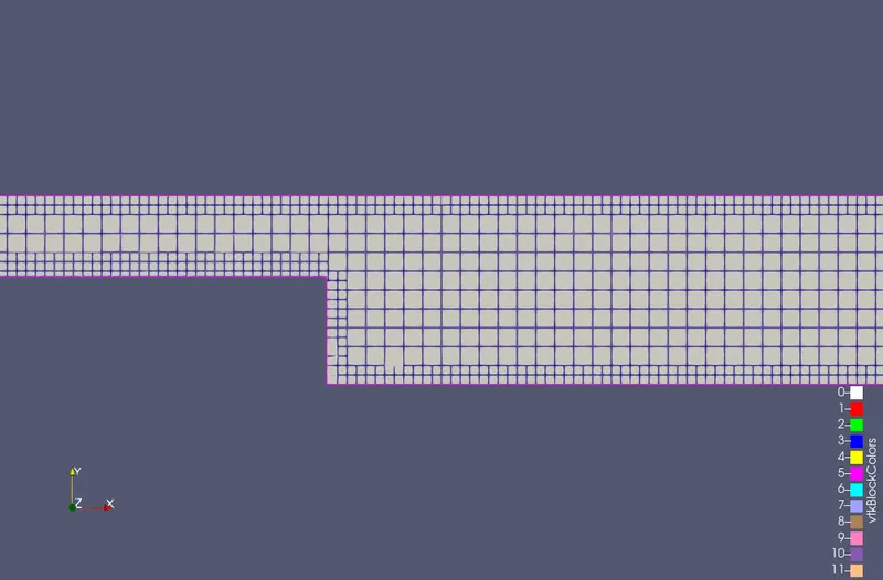
Mesh:
Mass Flow Rate:
Pressure:
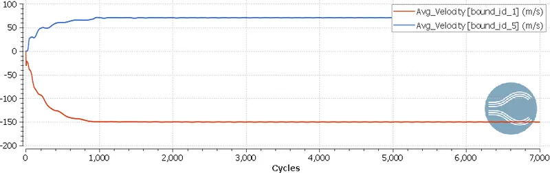
Velocity:
Total Cell Count:
Velocity Contour:
Pressure Contour:
Grid_2:
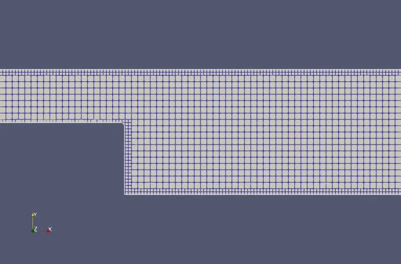
Mesh:
Mass Flow Rate:
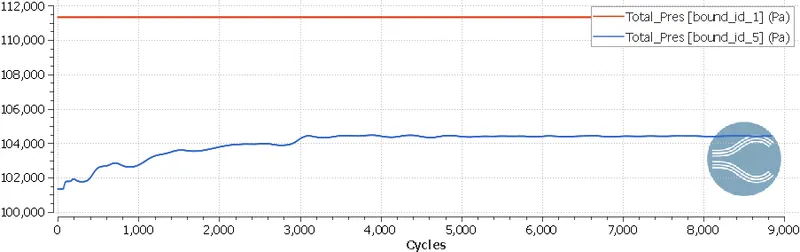
Pressure:
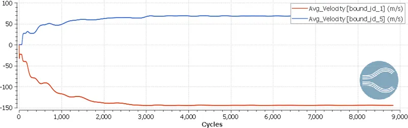
Velocity:
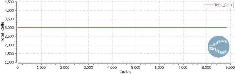
Total cell count:
Velocity Contour:
Pressure Contour:
Grid_3:
Mesh:
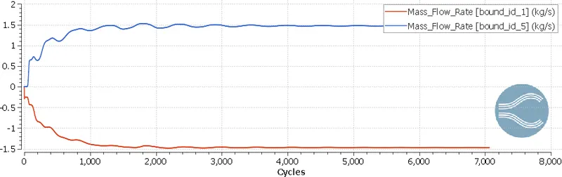
Mass Flow Rate:
Pressure:
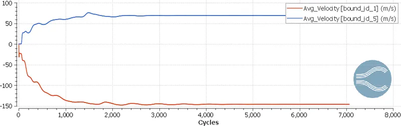
Velocity:
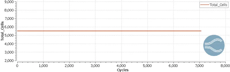
Total Cell Count:
Velocity Contour:
Pressure Contour:
Observations:
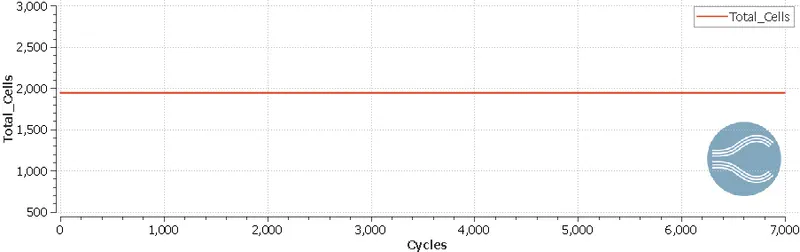
- From the simulation performed for mesh size (2e-4, 1.5e-4, 1.0e-4) the total cell count for each of the mesh is 2000, 3000, and 5500, respectively. Hence as the mesh becomes finer and finer the total cell count increases, and as the cell count increases the computational time also increases.
- It is observed that velocity in the initial case is highest but as the mesh is coarse it is not preferred to be accurate. In the next two cases, it is calculated more accurately.
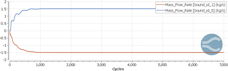
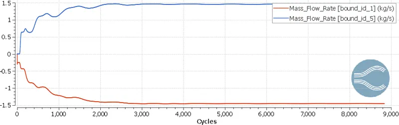
- The mass Flow Rate at the outlets for the refined cases is the same. When both inlets and outlets are compared, we can observe a positive and a negative flow.
- As the mesh becomes finer, the velocity profile obtained is also much clearer compared to the other two cases.
- Hence, as the size increases the results obtained are much clearer and more accurate
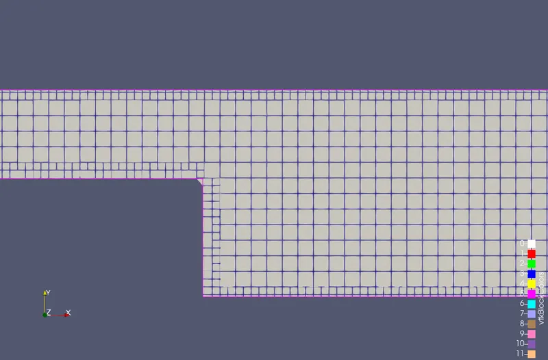
- The mesh at the wall boundary is finer due to the embedded meshing option with the scale of 1.
Conclusion:
The flow backward facing step was simulated using converge CFD with different mesh sizes and results are plotted