Week 9 - FVM Literature Review
Aim: Differentiate FVM and FDM and describe the need for interpolation schemes and flux limiters in FVM.
FVM: Finite Volume Method is a discretization method to evaluate the partial differential equation in the form of algebraic equations. It approximates through the control volumes and calculates the flux of the parameters through conservation laws applied to the PDEs.
Finite volume' refers to the small volume surrounding each node point on a mesh.
The advantage of the finite volume method is that it is easily formulated to allow unstructured meshes and this method is used in many computational fluid dynamic packages.
Flow quantities are conserved in the control volume
To solve a problem through FVM governing equations are solved over a finite volume and the gauss divergence theorem is applied to find the flux over the control volume. By using interpolation techniques face averaged values are approximated.
Difference between FVM and FDM:
- Governing equations are in differential form in FDM and integral form in FVM
- Equations are solved over the mesh points in the FDM whereas in FVM it is solved over the finite volume.
- Structured mesh in FDM and unstructured mesh in FVM
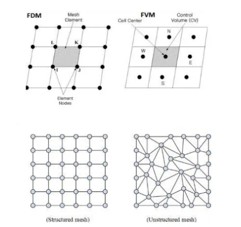
- The accuracy of the solution depends on the order of the discretization of the governing equations in FDM and in FVM the higher order solution will be highly complex.
- Conservation condition is not required in FDM whereas in FVM conservation condition is met at every cell and domain level.
Interpolation Scheme: These schemes are used to evaluate the face values of a control volume by using the neighbouring nodes.
Types of Interpolation Schemes:
- Upwind Interpolation scheme
- Linear Interpolation scheme
- Quadratic upwind interpolation scheme
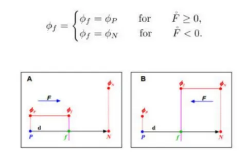
Upwind Interpolation Scheme:
It is used to calculate the approximate value based on the direction of flow with diffusive and convective character. It is first oreder accurate interpolation scheme.
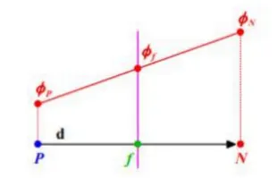
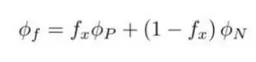
Linear Interpolation Scheme:
The face values are computed as a liner interpolation from the computational value and the neighbouring value. It is a second order accurate interpolation scheme.
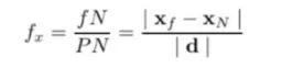
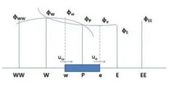
Quadratic Upwind Interpolation Scheme:
The face values are calculated by the quadratic equation by using three points (two surrounding nodes and one upstream node). It is a third order accuracy.

Flux Limiters: While solving using second or higher order interpolation schemes, will predict the face values using gradient of the cell node. Sometimes the value will overshoot these face values might exceed local maximum/minimum.
This overshooting of gradients causes the new maxima or minima which will leads to the instability.
The flux limiter function involved determining the ratio of successive gradients and, when it notices strong gradients, switches to the first order scheme locally.