Week 5.1 - Mid term project - Solving the steady and unsteady 2D heat conduction problem

Objective:

To solve the 2D heat conduction equation in a steady and unsteady state with different solving techniques i.e., Jacobi, Gauss-seidel and Successive over relaxation with implicit and explicit equations.

Boundary Conditions:

Top boundary condition = 600 K

Bottom boundary condition = 900 K

Right boundary condition = 800 K

Left boundary condition = 400 K

Assumptions:

1. Considering the square plate of length 1*1 m
2. The number of grid points on the X-axis and Y-axis is equal nx=ny
3. The number of grid points is nx=ny = 200
4. The initial temperature is 400K as there is no diffusion below the least boundary temperature
5. Tolerance is `10^-4`

Theory:

The differential equation of the heat conduction describes the temperature variation through the medium with respect to the position i.e., x,y- axis and the time i.e., t.

The equation of the 2-D heat conduction is `(deltaT)/(deltat) = alpha*((delta^2T)/(deltax^2) + (delta^2T)/(deltay^2))`

whereas `alpha` is the diffusivity of the medium

T is temperature

t is time

x,y are the space coordinates

By solving the above equation, we will get the temperatures at the position

Methods:

There are several solvers that can be used to solve the discretised equation which is helpful to converge the solution quickly and accurately.

The Jacobi method will be solved with old iteration values at each iteration whereas the gauss-seidel uses the calculated values for the preceding iteration and the successive over-relaxation is used to increase the speed for both solvers by using the slope equation and the relaxation factor where the relaxation factor decides the speed and iteration step.

Though the Jacobi solver takes greater iterations than the gauss-seidel than the successive over-relaxation solver.

Steady State solution:

Main code:

clear all
close all
clc

T_top = 600; %Boundary Conditions at top side
T_right = 800; %Boundary Conditions at right side 
T_bottom = 900; %Boundary Conditions at bottom side
T_left = 400; %Boundary Conditions at left side

x_length = 1; %X axis length of the plate
y_length = 1; %Y axis length of the plate

nx = 200; %X-axis grid points
ny = nx; %Y-axis grid points

T = 400*ones(ny,nx); %Intializing the temperature 

T(1,:)= T_top;      %Boundary conditions to the temperature matrix
T(end,:) = T_bottom; %Boundary conditions to the temperature matrix
T(:,1)= T_left; %Boundary conditions to the temperature matrix
T(:,end) = T_right; %Boundary conditions to the temperature matrix

T(1,1) = (T_top + T_left)/2; %Calculating temperature at the top left edge point 
T(1,end) = (T_top + T_right)/2; %Calculating temperature at the top right edge point
T(end,1) = (T_left+T_bottom)/2; %Calculating temperature at the bottom left edge point
T(end,end) = (T_right + T_bottom)/2; %Calculating temperature at the bottom right edge point

Told = T; %Told matrix

x = linspace(0,x_length,nx);  %X Grid points 
delx = x(2) - x(1); %change x

y = linspace(0,y_length,ny); %Y grid points
dely = y(2) - y(1); %change y

iterative_solver = 3; %Iterative solver 
tol = 1e-4; %Tolerence

if iterative_solver == 1
    tic;
    [T,iter,title_t] = jacobi_solver(tol,delx,dely,nx,ny,Told); %Jacobi solver 
    time = toc;
elseif iterative_solver == 2
    tic;
    [T,iter,title_t] = gauss_seidel_solver(tol,delx,dely,nx,ny,Told); %Gauss seidel solver
    time = toc;
elseif iterative_solver == 3
    tic;
    alpha = 1.3; %SOR Factor
    [T,iter,title_t] = sor_solver(tol,alpha,delx,dely,nx,ny,Told); %Succesive over relaxation 
    time = toc;
end

[c,v] = contourf(x,y,T,'LineWidth',0.1);  %Contour Plot
set(gcf, 'Position',  [500, 30, 750, 750]) %Position of the plot
set(gca, 'ydir', 'reverse')
colormap(jet); 
colorbar
axis('on', 'image');
title_text = sprintf('2D Heat Conduction by %s \n %d Iterations',title_t,iter); %Title of the text
title(title_text, 'FontSize', 15);
xlabel('x', 'FontSize', 15); %X-axis label
ylabel('y', 'FontSize', 15); %Y-axis label
clabel(c,v) %Labelling the points

Jacobi function:

function [T,iter,title_t] = jacobi_solver(tol,delx,dely,nx,ny,Told)

iter = 1; %Number of Iterations 
error = 1; %error intiation
T = Told; %Temperature matrix

while(error>tol) %error loop 
    k = 2*(((delx^2)+(dely^2))/((delx^2)*(dely^2))); %constant
    for i = 2: nx-1 %x-axis loop
        for j = 2:ny-1 %y-axis loop
            %T(i,j) =[2*(dx^2+dy^2)/(dx^2*dy^2)]*[((T(i+1,j)+T(i-1,j))/dx^2)+((T(i,j+1)+T(i,j-1))/dy^2)]
            term1 = (Told(i+1,j) + Told(i-1,j))/(delx^2); 
            term2 = (Told(i,j+1) + Told(i,j-1))/(dely^2);
            T(i,j) = (term1 + term2)/k;
        end
    end
    error = max(abs(Told - T),[],'all'); %error calculation
    Told = T; %changing the old temperature matrix
    iter = iter+1; %increasing the number of iterations
    title_t = 'Jacobi Method'; %title of the solver
end

end

Gauss-Seidel Function:

function [T,iter,title_t] = gauss_seidel_solver(tol,delx,dely,nx,ny,Told)

iter = 1; %Number of Iterations
error=1; %error intiation
T = Told; %Teperature matrix

while(error>tol) %error loop
    k = 2*(((delx^2)+(dely^2))/((delx^2)*(dely^2))); %constant
    for i = 2: nx-1 %x-axis loop
        for j = 2:ny-1 %y-axis loop
            %T(i,j) =[2*(dx^2+dy^2)/(dx^2*dy^2)]*[((T(i+1,j)+T(i-1,j))/dx^2)+((T(i,j+1)+T(i,j-1))/dy^2)]
            term1 = (T(i+1,j) + T(i-1,j))/(delx^2);
            term2 = (T(i,j+1) + T(i,j-1))/(dely^2);
            T(i,j) = (term1 + term2)/k;
        end
    end
    error = max(abs(Told - T),[],'all'); %error Calculation
    Told = T; %changing the old temperature matrix
    iter = iter+1; %increasing the number of iterations
    title_t = 'Gauss-Seidel Method'; %title of the solver
end

end

Successive Over Relaxation Function:

function [T,iter,title_t] = sor_solver(tol,alpha,delx,dely,nx,ny,Told)

iter = 1; %Number of Iterations
error=1; %error intiation
T = Told; %Teperature matrix

while(error>tol) %error loop
    k = 2*(((delx^2)+(dely^2))/((delx^2)*(dely^2))); %constant
    for i = 2: nx-1 %x-axis loop
        for j = 2:ny-1 %y-axis loop
            %T(i,j) =[2*(dx^2+dy^2)/(dx^2*dy^2)]*[((T(i+1,j)+T(i-1,j))/dx^2)+((T(i,j+1)+T(i,j-1))/dy^2)]
            term1 = (T(i+1,j) + T(i-1,j))/(delx^2);
            term2 = (T(i,j+1) + T(i,j-1))/(dely^2);
            Tgs(i,j) = (term1 + term2)/k;
            T(i,j) = ((1-alpha)*(Told(i,j))) + (alpha*Tgs(i,j));
        end
    end
    error = max(abs(Told - T),[],'all'); %error calculation
    Told = T; %changing the old tempertaure matrix
    iter = iter+1; %increasing the number of iterations
    title_t = 'Succesive Over Relaxation Method'; %title of the solver
end

end

Steady-state condition is where the temperature is the same with respect to the time

so, the term `(deltaT)/(deltat) = 0`

and the equation for steady state is `((delta^2T)/(deltax^2) + (delta^2T)/(deltay^2)) = 0`

By discretizing

`((T_(i+1,j) - 2*T_(i,j)+T_(i-1,j))/(Deltax^2))^n + ((T_(i,j+1) - 2*T_(i,j)+T_(i,j-1))/(Deltay^2))^n = 0`

by solving

`T_(i,j) =1/ k*(((T_(i+1,j) + T_(i-1,j))/(Deltax^2)) + ((T_(i,j+1) + T_(i,j-1))/(Deltay^2) ))`

`k = (2*(Deltax^2+Deltay^2)/(Deltax^2*Deltay^2))`

This equation can be solved with three methods Jacobi, Gauss-seidel and Successive over Relaxation

Steady-state solution by Jacobi method:

The discretized equation will be `T_(i,j) =1/ k*(((Told_(i+1,j) + Told_(i-1,j))/(Deltax^2)) + ((Told_(i,j+1) + Told_(i,j-1))/(Deltay^2)))`

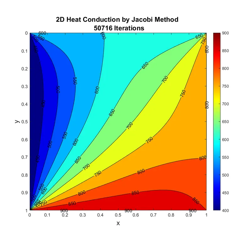
This solver took 50716 iterations to solve the problem

Steady-state solution by Gauss-seidel method:

The discretized equation will be `T_(i,j) =1/ k*(((Told_(i+1,j) + T_(i-1,j))/(Deltax^2)) + ((Told_(i,j+1) + T_(i,j-1))/(Deltay^2)))`

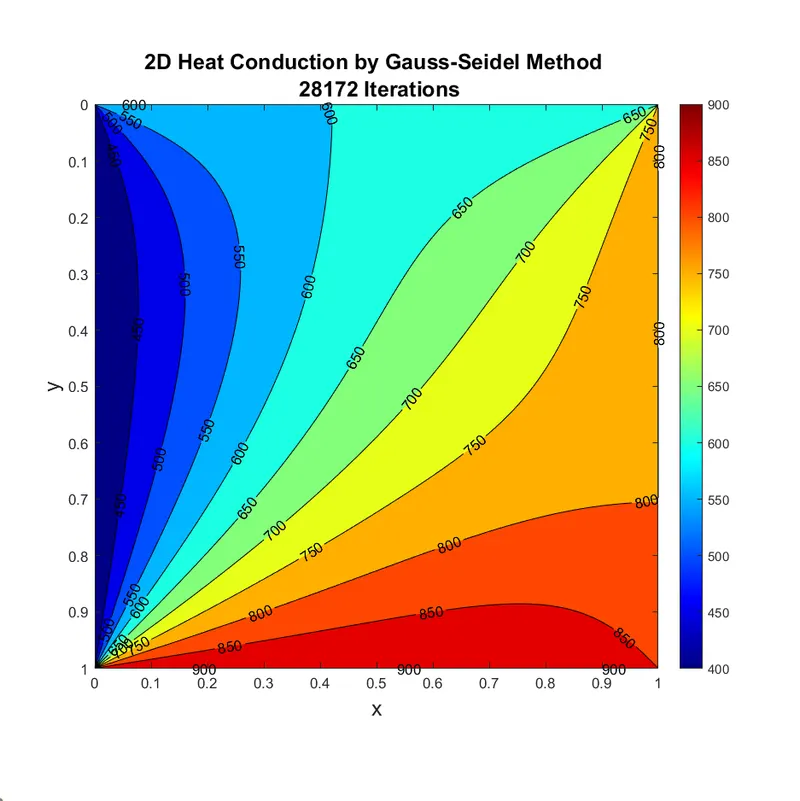
The solver took 28172 iterations to solve the equation

Steady-state solution by Successive Over Relaxation method:

The discretized equation will be

`Tgs_(i,j) = (1/k)*((T_(i+1,j) + T_(i-1,j))/(Deltax^2) + (T_(i,j+1) + T_(i,j-1))/(Deltay^2))`

`T_(i,j) = ((1-alpha)*Told_(i,j)) + (alpha*Tgs_(i,j))`

where `alpha` is the relaxation factor which is 1.5.

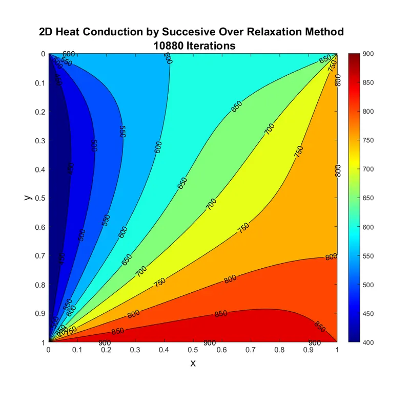
The solver took 10880 iterations to solve the equation.

Transient condition:

The transient condition is solved with implicit and explicit equations

Transient Condition solved explicitly:

The discretized equation `T_(i,j)^(n+1) = (T_(i,j)^(n)*(1 - 2k_1 - 2k_2)) + (k_1*(T_(i+1,j)^n+T_(i-1,j)^n)) + (k_2*(T_(i,j+1)^n+T_(i,j-1)^n))`

where `k_1 = (alpha*Deltat)/(Deltax^2)`

`k_2 = (alpha*Deltat)/(Deltay^2)`

where the `CFL = k_1 + k_2`

`CFL <= 0.5` for the valid solution

So, the values of the diffusivity and the `Delta t` and `Deltax, Deltay` are considered carefully within the condition

Code:

clear all
close all
clc

T_top = 600; %Boundary Conditions at top side
T_right = 800; %Boundary Conditions at right side 
T_bottom = 900; %Boundary Conditions at bottom side
T_left = 400; %Boundary Conditions at left side

x_length = 1; %X axis length of the plate
y_length = 1; %Y axis length of the plate

nx = 100; %X-axis grid points
ny = nx; %Y axis grid points
t = 1000; %time

T = 400*ones(ny,nx); %Intializing the temperature 

T(1,:)= T_top; %Boundary conditions to the temperature matrix
T(end,:) = T_bottom; %Boundary conditions to the temperature matrix
T(:,1)= T_left; %Boundary conditions to the temperature matrix
T(:,end) = T_right; %Boundary conditions to the temperature matrix

T(1,1) = (T_top + T_left)/2;  %Calculating temperature at the top left edge point 
T(1,end) = (T_top + T_right)/2; %Calculating temperature at the top right edge point
T(end,1) = (T_left+T_bottom)/2; %Calculating temperature at the bottom left edge point
T(end,end) = (T_right + T_bottom)/2; %Calculating temperature at the bottom right edge point

Told = T;%Told matrix

x = linspace(0,x_length,nx); %X Grid points
delx = x(2) - x(1); %Change x

y = linspace(0,y_length,ny); %Y Grid points
dely = y(2) - y(1); %Change y

delt = 0.00001; %Change time
nt = 0:delt:t; %Time step


tol = 1e-4; %Tolerance
error = 1; %Error intiation
iter = 1; %Number  of iterations
alpha = 1.2 ; %Coefficient

k1 = (alpha*delt)/(delx^2); %Constants
k2 = (alpha*delt)/(dely^2); %Constants

cfl = ((alpha*delt)/(delx^2))+((alpha*delt)/(dely^2));

tic;
for it = 1:length(nt) %Time loop
    while error > tol %Convergence loop
        for i = 2:nx-1 %X axis loop
            for j = 2:ny-1 %Y axis loop
                term1 = (Told(i,j)*(1-(2*k1)-(2*k2)));
                term2 = (k1*(Told(i+1,j)+Told(i-1,j)));
                term3 = (k2*(Told(i,j+1)+Told(i,j-1)));
                T(i,j) = term1 + term2 + term3;                                     
            end
        end
        error = max(abs(Told - T),[],'all'); %error 
        Told = T; %Updating the t old matrix
        iter = iter+1; %Increasing the number of iterations
    end
end
time=toc;

[c,v] = contourf(x,y,T,'LineWidth',0.1); %Contour Plot
clabel(c,v)
set(gcf, 'Position',  [500, 30, 750, 750]) %Positionof the plot
set(gca,'ydir','reverse')
colormap(jet);
colorbar
axis('on', 'image');
title_text = sprintf('2D Transient Heat Conduction solved explicitly \n %d Iterations',iter);
title(title_text, 'FontSize', 15);
xlabel('x', 'FontSize', 15); %Xlabel
ylabel('y', 'FontSize', 15); %Ylabel

Output:

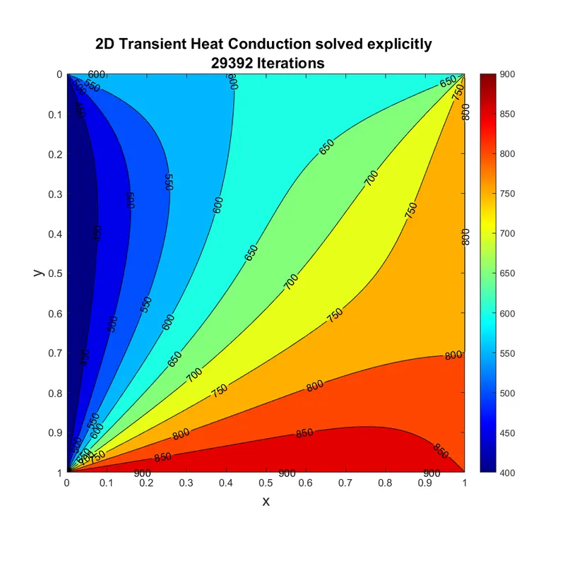
Through implicit equations, the solution is converged after 29392 iterations.

Transient condition solved implicitly:

The discretized `T_(i,j)^(n+1) = (T_(i,j)^(n)*(1 - 2k_1 - 2k_2)) + (k_1*(T_(i+1,j)^(n+1)+T_(i-1,j)^(n+1))) + (k_2*(T_(i,j+1)^(n+1)+T_(i,j-1)^(n+1)))`

where `k_1 = (alpha*Deltat)/(Deltax^2)`

`k_2 = (alpha*Deltat)/(Deltay^2)`

Main code:

clear all
close all
clc

T_top = 600; %Boundary Conditions at top side
T_right = 800; %Boundary Conditions at right side 
T_bottom = 900; %Boundary Conditions at bottom side
T_left = 400; %Boundary Conditions at left side

x_length = 1; %X axis length of the plate
y_length = 1; %Y axis length of the plate

nx = 100; %X-axis grid points
ny = nx; %Y axis grid points
t = 1400; %time

T = 400*ones(ny,nx); %Intializing the temperature 

T(1,:)= T_top; %Boundary conditions to the temperature matrix
T(end,:) = T_bottom; %Boundary conditions to the temperature matrix
T(:,1)= T_left; %Boundary conditions to the temperature matrix
T(:,end) = T_right; %Boundary conditions to the temperature matrix

T(1,1) = (T_top + T_left)/2;  %Calculating temperature at the top left edge point 
T(1,end) = (T_top + T_right)/2; %Calculating temperature at the top right edge point
T(end,1) = (T_left+T_bottom)/2; %Calculating temperature at the bottom left edge point
T(end,end) = (T_right + T_bottom)/2; %Calculating temperature at the bottom right edge point

Told = T; %Told matrix

x = linspace(0,x_length,nx); %X Grid points
delx = x(2) - x(1); %Change x

y = linspace(0,y_length,ny); %Y Grid points
dely = y(2) - y(1); %Change y

delt = 1; %Change time
nt = 0:delt:t; %Time step

tol = 1e-4; %Tolerance
alpha =1.2 ; %Coefficient
iterative_solver = 1; %Solver selection

k1 = (alpha*delt)/(delx^2); %Constants
k2 = (alpha*delt)/(dely^2); %Constants
term1 = 1/(1+(2*k1)+(2*k2));
term2 = k1*term1;
term3 = k2*term1;

cfl = ((alpha*delt)/(delx^2))+((alpha*delt)/(dely^2));

if iterative_solver == 1
    tic;
    [T,iter,title_t] = transient_jacobi_solver(term1,term2,term3,tol,nt,nx,ny,Told); %Jacobi solver 
    time = toc;
elseif iterative_solver == 2
    tic;
    [T,iter,title_t] = transient_gauss_seidel_solver(term1,term2,term3,tol,nt,nx,ny,Told); %Gauss seidel solver
    time = toc;
elseif iterative_solver == 3
    tic;
    [T,iter,title_t] = transient_sor_solver(term1,term2,term3,tol,nt,nx,ny,Told); %Succesive over relaxation 
    time = toc;
end

[c,v] = contourf(x,y,T,'LineWidth',0.1);  %Contour Plot
set(gcf, 'Position',  [500, 30, 750, 750]) %Position of the plot
set(gca,'ydir','reverse')
colormap(jet); 
colorbar
axis('on', 'image');
title_text = sprintf('2D Heat Conduction by %s \n %d Iterations',title_t,iter); %Title of the text
title(title_text, 'FontSize', 15);
xlabel('x', 'FontSize', 15); %X-axis label
ylabel('y', 'FontSize', 15); %Y-axis label
clabel(c,v) %Labelling the points

Jacobi Function:

function [T,iter,title_t] = transient_jacobi_solver(term1,term2,term3,tol,nt,nx,ny,Told)

iter = 1; %Number of Iterations 
error = 1; %error intiation
T_initial = Told; %Temperature matrix
T = Told;
title_t = 'Jacobi Method'; %title of the solver

for it = 1:length(nt)
    while error > tol  %error loop 
        for i = 2:nx-1 %x-axis loop
            for j = 2:ny-1 %y-axis loop
                H = (Told(i+1,j)+Told(i-1,j));
                V = (Told(i,j+1)+Told(i,j-1));   
                T(i,j) = ((T_initial(i,j))*term1)+(H*term2)+(V*term3);
            end
        end
        error = max(abs(Told - T),[],'all'); %error calculation
        Told = T; %changing the old temperature matrix
        iter = iter+1; %increasing the number of iterations
    end
    T_initial = T;
end

end

Gauss-Seidel Function:

function [T,iter,title_t] = transient_gauss_seidel_solver(term1,term2,term3,tol,nt,nx,ny,Told)

iter = 1; %Number of Iterations 
error = 1; %error intiation
T_initial = Told; %Temperature matrix
T = Told;
title_t = 'Gauss Seidel Method'; %title of the solver

for it = 1:length(nt)
    while error > tol  %error loop 
        for i = 2:nx-1 %x-axis loop
            for j = 2:ny-1 %y-axis loop
                H = (T(i+1,j)+T(i-1,j));
                V = (T(i,j+1)+T(i,j-1));   
                T(i,j) = ((T_initial(i,j))*term1)+(H*term2)+(V*term3);
            end
        end
        error = max(abs(Told - T),[],'all'); %error calculation
        Told = T; %changing the old temperature matrix
        iter = iter+1; %increasing the number of iterations
    end
    T_initial = T;
end

end

Successive Over Relaxation:

function [T,iter,title_t] = transient_sor_solver(term1,term2,term3,tol,nt,nx,ny,Told)

iter = 1; %Number of Iterations 
error = 1; %error intiation
T_initial = Told; %Temperature matrix
T = Told;
Tgs = Told;
title_t = 'Successive Over Relaxation Method'; %title of the solver
beta = 1.3;

for it = 1:length(nt)
    while error > tol  %error loop 
        for i = 2:nx-1 %x-axis loop
            for j = 2:ny-1 %y-axis loop
                H = (T(i+1,j)+T(i-1,j));
                V = (T(i,j+1)+T(i,j-1));   
                Tgs(i,j) = ((T_initial(i,j))*term1)+(H*term2)+(V*term3);
                T(i,j) = ((1-beta)*Told(i,j)) + (beta*Tgs(i,j));
            end
        end
        error = max(abs(Told - T),[],'all'); %error calculation
        Told = T; %changing the old temperature matrix
        iter = iter+1; %increasing the number of iterations
    end
    T_initial = T;
end

end

Output:

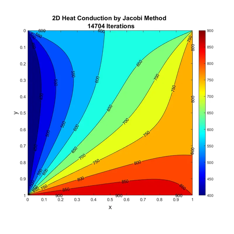
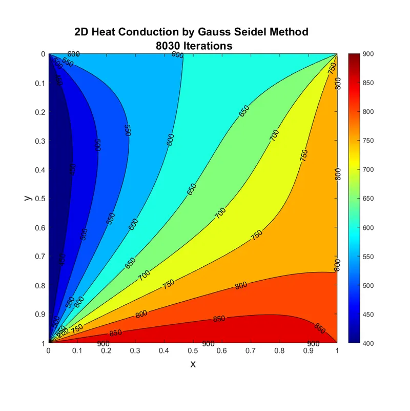
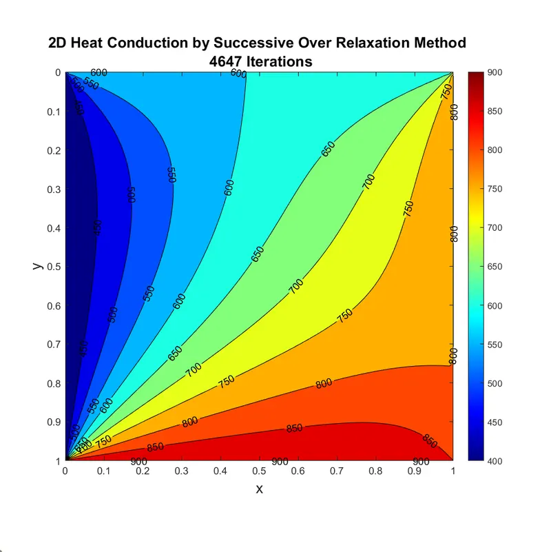
Conclusion:

The 2D heat conduction is solved in a steady-state and unsteady state with implicit and explicit solved with Jacobi, Gauss-seidel and Successive over Relaxation solver

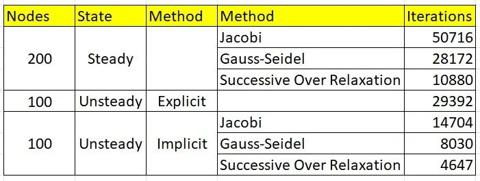
This solution concludes that iterations Successive Over relaxation < Gauss-Seidel < Jacobi in any case

In unsteady explicit conditions, CFL is k1+k2 which has to be less than 0.5 for the steady and accurate solution