Week 5 - Genetic Algorithm

STALAGMITE FUNCTION:

`f(x,y) = -f_(1,x)*f_(1,y)*f_(2,x)*f_(2,y)`

where,

`f_(1,x) = [sin(5.1*pi*x) + 0.5]^6`

`f_(1,y) = [sin(5.1*pi*y) + 0.5]^6`

`f_(2,x) = exp[-4*ln(2)*((x-0.0667)^2/0.64)]`

`f_(2,y) = exp[-4*ln(2)*((y-0.0667)^2/0.64)]`

Negative sign is introduced to find the maximum value

GENETIC ALGORITHM:

A genetic algorithm is a method to solve the optimization problem based on the natural selection process. It uses the genetic modulating method to create the next generation of points to find the global maxima. It initially has a random population to solve the optimization than by using the biological genetics creation method to increase the search area to find the local maxima. The generation evolves in three steps selection, crossover, and mutation. The genetic algorithm randomly selects individuals from the current population and uses them as parents to produce children for the next generation. Crossover is applied probabilistically for each pair of parents, meaning that in some cases, copies of the parents are taken as the children instead of the recombination operator.

SYNTAX:

[x,fval] = ga(fun,nvars,A,b,Aeq,beq,lb,ub,nonlcon,intcon,options)

x = input values of objective function

fval = fitness values

fun = Objective function

nvars = Number of variables

A, Aeq = Linear inequality constraints coefficients

b, beq = Linear inequality constraints

lb = Lower bound

ub = Upper bounds

nonlcon = Non linear constraints

intcon = integer constraints

options = options to increase the efficiency of the code

CODE EXPLANATION:

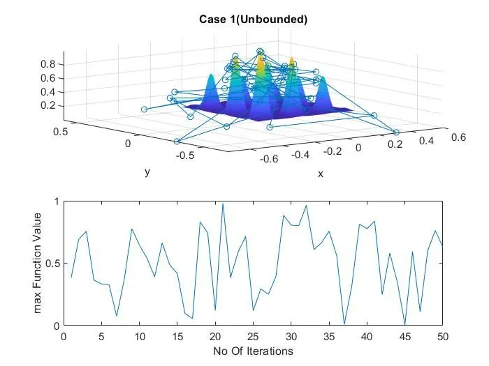
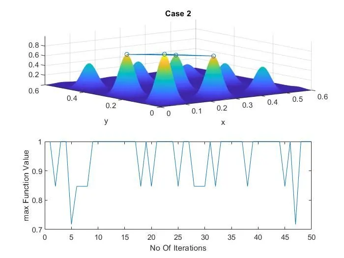
Initially, the code started with creating an array of x and y elements and limiting values of the number of iterations that the genetic algorithm performs, then creating a mesh grid for the x and y elements. The stalagmite function is used to find the solution of the mesh grid values. Then the code is divided into three cases Case 1: no bound for executing the genetic algorithm, Case 2: with the bound of input values from 0-0.6 then Case 3: With a population size of 250. For each case, the function is executed for 50 times to check for the same solution at each time which was succeeded in case 3. 'Surfc' function is used to plot the function values with surface contour and the input values for the genetic algorithm. and another plot is made between a number of iterations and function values for each case.

MAIN FUNCTION:

%Start of program
clear all
close all
clc

stalag_f = @stalagmite_function;

x = linspace(0,0.6,150);
y = linspace(0,0.6,150);
limit = 50;

%Creating 2D array
[xx, yy] = meshgrid(x,y);

%Loop for array value input
for i = 1:length(xx)
    for j = 1:length(yy)
        in_v(1) = xx(i,j);
        in_v(2) = yy(i,j);
        f(i,j) = stalagmite_function(in_v);
    end
end

%Case 1 
tic
for i = 1:limit

    [input_case_1,f_val_case_1(i)] = ga(stalag_f,2);
    x_input_case_1(i) = input_case_1(1);
    y_input_case_1(i) = input_case_1(2);

end
time_case_1 = toc;

figure(1)
subplot(2,1,1)
surfc(xx,yy,-f)          %Creating contour plot 
xlabel('x')
ylabel('y')
title('Case 1(Unbounded)','color','k')
shading interp
hold on;
plot3(x_input_case_1,y_input_case_1,-f_val_case_1,'marker','o','MarkerSize',5);
subplot(2,1,2)
plot(-f_val_case_1);     %Plotting function values at different iterations
xlabel('No Of Iterations')
ylabel('max Function Value')

%Case 2
tic
for i = 1:limit

    [input_case_2,f_val_case_2(i)] = ga(stalag_f,2,[],[],[],[],[0;0],[0.6;0.6]);
    x_input_case_2(i) = input_case_2(1);
    y_input_case_2(i) = input_case_2(2);

end
time_case_2 = toc;

figure(2)
subplot(2,1,1)
surfc(xx,yy,-f)
xlabel('x')
ylabel('y')
title('Case 2','color','k')
shading interp
hold on;
plot3(x_input_case_2,y_input_case_2,-f_val_case_2,'marker','o','MarkerSize',5);
subplot(2,1,2)
plot(-f_val_case_2);
xlabel('No Of Iterations')
ylabel('max Function Value')

%Case 3
tic
options = optimoptions('ga','PopulationSize',250);

for i = 1:limit

    [input_case_3,f_val_case_3(i)] = ga(stalag_f,2,[],[],[],[],[0;0],[0.6;0.6],[],[],options);
    x_input_case_3(i) = input_case_3(1);
    y_input_case_3(i) = input_case_3(2);

end
time_case_3 = toc;

figure(3)
subplot(2,1,1)
surfc(xx,yy,-f)
xlabel('x')
ylabel('y')
title('Case 3','color','k')
shading interp
hold on;
plot3(x_input_case_3,y_input_case_3,round(-f_val_case_3,5),'marker','o','MarkerSize',5);
subplot(2,1,2)
plot(round(-f_val_case_3,5));
xlabel('No Of Iterations')
ylabel('max Function Value')

STALAGMITE FUNCTION:

function [f] = stalagmite_function(in_v)

    f_1_x = (sin((5.1*pi*in_v(1))+0.5))^6;
    f_1_y = (sin((5.1*pi*in_v(2))+0.5))^6;

    f_2_x = exp(-4*log(2)*((in_v(1)-0.0667)^2)/0.64);
    f_2_y = exp(-4*log(2)*((in_v(2)-0.0667)^2)/0.64);

    f = -f_1_x*f_2_x*f_1_y*f_2_y;

end

RESULT:

CASE 1:

CASE 2:

CASE 3:

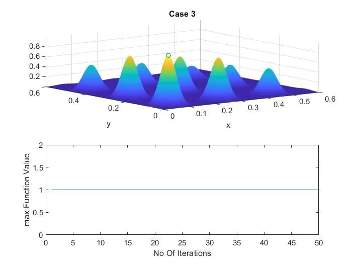
The global maxima is attained at [0.0668,0.0668] and the function value is 1

In case 1 the genetic algorithm searches all over the field where there are no bounds so the solution is different at each iteration but in case 2 with upper and lower bounds the results are confined within the limits. In case 3 with the limit in population size to 250 genetic algorithm found global maxima which are the same at every iteration.