Week 7 - Simulation of a 1D Super-sonic nozzle flow simulation using Macormack Method
Objective:
To simulate the isentropic flow through a quasi 1D subsonic-supersonic nozzle. To derive in both the conservative and non-conservative forms of the governing equations by solving using MacCormark's technique.
Aim:
- To plot the steady-state distribution of primitive variables inside the nozzle
- To plot the time-wise variation of the primitive variables
- Variation of Mass flow rate distribution inside the nozzle at different time steps during the time-marching process
- To compare Normalized mass flow rate distributions of both forms
Theory:
The numerical solution of the quasi-static 1D supersonic nozzle flow with MacCormack technique. Primitive variables are calculated by the governing equations like density by the continuity equation, velocity by the momentum equation and temperature by the energy equation. The numerical solution is not as exact as the analytical solution but can get nearly to the solution with the grid point variation and time marching steps.
Nozzle Diagram:
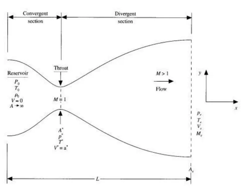
Governing Equations:
Non-Conservative Form:
Continuity Equation: `(del(rhoA))/(delt) + rhoA(delV)/(delx) + rhoV(delA)/(delx) + VA(delrho)/(delx) = 0`
Momentum Equation: `rho(delV)/(delt) + rhoV(delV)/(delx) = -R(rho(delT)/(delx) + T(delrho)/(delx))`
Energy Equation: `rhoc_v(delT)/(delt) + rhoVc_v(delT)/(delx) = - rhoRT[(delV)/(delx) + V(del(ln A))/(delx)]`
Conservative Form:
Continuity Equation: `(del(rho'A'))/(delt') + (del(rho'A'V'))/(delx') = 0`
Momentum Equation: `(del(rho'A'V'))/(delt') +(del[rho'A'V'^2 + (1/gamma)p'A'])/(delx') = 1/gamma p'(delA')/(delx')`
Energy equation: `(del[rho'((e')/(gamma-1)) + gamma/2V'^2)A']/(delt') + (del[rho'((e')/(gamma-1) + gamma/2V'^2)V'A' + p'A'V'])/(delx') = 0`
MacCormack Technique:
This technique consists of three parts first to calculate the rate of change of value through the predictor step then update the values and then calculate through corrector step then the values are averaged to get the final change value then the next value is calculated using the average value
In the predictor step the forward difference method is used whereas in the corrector step backward difference method is used.
Program Logic:
The program consists of three parts 1. Main program 2. Function for Nonconservative form 3. Function for conservative form
The input variables are time total time, length and number of grid points and courant number.
The plots are made between the values of primitive variables and the nozzle length
Main:
clear all
close all
clc

%Solving Quasi 1D supersonic nozzle flow equations

nt = 600;   %Time
l = 3;     %Length
n = 31;    %Number of grid points
C = 0.5;   %Courant Number
x = linspace(0,l,n);  %Length meshed

%Nonconservative Function
[v_nonconservative,rho_nonconservative,T_nonconservative,m_nonconservative,M_nonconservative,P_nonconservative] = nonconservative_function(n,l,nt,C);

%Conservative function
[v_conservative,rho_conservative,T_conservative,m_conservative,M_conservative,P_conservative] = conservative_function(n,l,nt,C);

figure(5)
sp1 = subplot(3,2,1);
plot(x,v_nonconservative)
title('Velocity')
xlabel('Nozzle Length')
ylabel('Velocity')
sp2 = subplot(3,2,2);
plot(x,rho_nonconservative)
title('Density')
xlabel('Nozzle Length')
ylabel('Density')
sp3 = subplot(3,2,3);
plot(x,T_nonconservative)
title('Temperature')
xlabel('Nozzle Length')
ylabel('Temperature')
sp4 = subplot(3,2,4);
plot(x,m_nonconservative)
title('Mass Flow Rate')
xlabel('Nozzle Length')
ylabel('Mass Flow Rate')
sp5 = subplot(3,2,5);
plot(x,M_nonconservative)
title('Mach number')
xlabel('Nozzle Length')
ylabel('Mach Number')
sp6 = subplot(3,2,6);
plot(x,P_nonconservative)
title('Pressure')
xlabel('Nozzle Length')
ylabel('Pressure')
xlim(sp1,[0 3]);
ylim(sp1,[0 2.25]);
xlim(sp2,[0 3]);
ylim(sp2,[0 1.5]);
xlim(sp3,[0 3]);
ylim(sp3,[0 1.25]);
xlim(sp4,[0 3]);
ylim(sp4,[0 2.5]);
xlim(sp5,[0 3]);
ylim(sp5,[0 6.5]);
xlim(sp6,[0 3]);
ylim(sp6,[0 1.5]);
sgtitle('Steady state Nonconservative Form primitive variables')

figure(6)
sp1 = subplot(3,2,1);
plot(x,v_conservative)
title('Velocity')
xlabel('Nozzle Length')
ylabel('Velocity')
sp2 = subplot(3,2,2);
plot(x,rho_conservative)
title('Density')
xlabel('Nozzle Length')
ylabel('Density')
sp3 = subplot(3,2,3);
plot(x,T_conservative)
title('Temperature')
xlabel('Nozzle Length')
ylabel('Temperature')
sp4 = subplot(3,2,4);
plot(x,m_conservative)
title('Mass Flow Rate')
xlabel('Nozzle Length')
ylabel('Mass Flow Rate')
sp5 = subplot(3,2,5);
plot(x,M_conservative)
title('Mach number')
xlabel('Nozzle Length')
ylabel('Mach Number')
sp6 = subplot(3,2,6);
plot(x,P_conservative)
title('Pressure')
xlabel('Nozzle Length')
ylabel('Pressure')
xlim(sp1,[0 3]);
ylim(sp1,[0 2.25]);
xlim(sp2,[0 3]);
ylim(sp2,[0 1.5]);
xlim(sp3,[0 3]);
ylim(sp3,[0 1.25]);
xlim(sp4,[0 3]);
ylim(sp4,[0 2.5]);
xlim(sp5,[0 3]);
ylim(sp5,[0 6.5]);
xlim(sp6,[0 3]);
ylim(sp6,[0 1.5]);
sgtitle('Steady state Conservative Form primitive variables')

figure(7)
title('Mass Flow Rate Comparision Plot')
plot(x,m_conservative,x,m_nonconservative,'linewidth',1.25)
legend('Conservative','Non Conservative')
xlabel('Nozzle Length')
ylabel('Mass Flow rate')
grid('on')
Non-Conservative:
The function calculates the Mach number, Pressure, Mass flow, Velocity and density across the nozzle at all grid points
Initial and final boundary are calculated by the values at next grid point
Firstly, the mesh is generated with the number of grid points and the length of nozzle then time step control is calculated. The time loop is started then predictor step is calculated then values are updated and then corrector step then the mean is taken and the next time step value is calculated. plots are made to get the change of variables throughout the time.
function [v,rho,T,m,M,P] = nonconservative_function(n,l,nt,C)

%Grid Points
x = linspace(0,l,n);
dx = x(2) - x(1);

%Constants
gamma = 1.4;

%Intial properties
A   = 1 + (2.2*((x - 1.5).^2));
rho = 1 - (0.3146*x);
T   = 1 - (0.2314*x);
v   = (0.1 + (1.09*x)).*(T.^0.5);

%Time step control
dt = min(C.*dx./(sqrt(T)+v));

fr = 1;

%Time Loop
for t = 1:nt

    %Grid points
    for j = 2 : n-1

        %Forward difference
        dv_dx_f = (v(j+1) - v(j))/dx  ;
        dA_dx_f = (log(A(j+1)) - log(A(j)))/dx ;
        drho_dx_f = (rho(j+1) - rho(j))/dx ;
        dT_dx_f = (T(j+1) - T(j))/dx ;

        %Backward difference
        dv_dx_b = (v(j) - v(j-1))/dx  ;
        dA_dx_b = (log(A(j)) - log(A(j-1)))/dx ;
        drho_dx_b = (rho(j) - rho(j-1))/dx ;
        dT_dx_b =  (T(j) - T(j-1))/dx ;

        %Predictor Step
        drho_dt_p = -(rho(j)*dv_dx_f)-(rho(j)*v(j)*dA_dx_f)-(v(j)*drho_dx_f);  %Continuity Equation
        dv_dt_p = -(v(j)*dv_dx_f)-(((dT_dx_f)+((T(j)/rho(j))*drho_dx_f))/gamma); %Momentum Equation
        dT_dt_p = -(v(j)*dT_dx_f)-(((dv_dx_f)+(v(j)*dA_dx_f))*((gamma-1)*T(j))); %Energy Equation

        %Solution Update
        rho_u = rho(j) + (drho_dt_p*dt);
        v_u = v(j) + (dv_dt_p*dt);
        T_u = T(j) + (dT_dt_p*dt);

        %Corrector Step
        drho_dt_c = -(rho_u*dv_dx_b)-(rho_u*v_u*dA_dx_b)-(v_u*drho_dx_b);  %Continuity Equation
        dv_dt_c = -(v_u*dv_dx_b)-(((dT_dx_b)+((T_u/rho_u)*drho_dx_b))/gamma); %Momentum Equation
        dT_dt_c = -(v_u*dT_dx_b)-(((dv_dx_b)+(v_u*dA_dx_b))*((gamma-1)*T_u)); %Energy Equation

        %Average
        drho_dt_avg = (drho_dt_p + drho_dt_c)/2;
        dv_dt_avg = (dv_dt_p + dv_dt_c)/2;
        dT_dt_avg = (dT_dt_p + dT_dt_c)/2;

        %Final Value
        rho(j) = rho(j) + (drho_dt_avg * dt);
        v(j) = v(j) + (dv_dt_avg * dt);
        T(j) = T(j) + (dT_dt_avg * dt);

    end

    %Boundary conditions Inlet
    v(1) = 2*v(2) - v(3);

    %Boundary Conditions Outlet
    v(n) = 2*v(n-1) - v(n-2);
    rho(n) = 2*rho(n-1) - rho(n-2);
    T(n) = 2*T(n-1) - T(n-2);

    %Calculating other variables
    m = rho .* A .* v;
    P = (rho .* T);
    M = (v./ sqrt(T)) ;

    %Mass Flow at different time steps
    if t == nt/5
        m_nt1 = m;
    elseif t == 2*nt/5
        m_nt2 = m;
    elseif t == 3*nt/5
        m_nt3 = m;
    elseif t == 4*nt/5
        m_nt4 = m;
    elseif t == nt
        m_nt5 = m;
    end

    %Plotting
    figure(1)
    set(gcf,'units','normalized','outerposition',[0 0.001 1 1])

    sp1 = subplot(3,2,1);
    plot(x,v)
    title('Velocity')
    xlabel('Nozzle Length')
    ylabel('Velocity')
    grid minor;
    sp2 = subplot(3,2,2);
    plot(x,rho)
    title('Density')
    xlabel('Nozzle Length')
    ylabel('Density')
    grid minor;
    sp3 = subplot(3,2,3);
    plot(x,T)
    title('Temperature')
    xlabel('Nozzle Length')
    ylabel('Temperature')
    grid minor;
    sp4 = subplot(3,2,4);
    plot(x,m)
    title('Mass Flow Rate')
    xlabel('Nozzle Length')
    ylabel('Mass Flow Rate')
    grid minor;
    sp5 = subplot(3,2,5);
    plot(x,M)
    title('Mach number')
    xlabel('Nozzle Length')
    ylabel('Mach Number')
    grid minor;
    sp6 = subplot(3,2,6);
    plot(x,P)
    title('Pressure')
    xlabel('Nozzle Length')
    ylabel('Pressure')
    grid minor;
    xlim(sp1,[0 3]);
    ylim(sp1,[0 2.25]);
    xlim(sp2,[0 3]);
    ylim(sp2,[0 1.5]);
    xlim(sp3,[0 3]);
    ylim(sp3,[0 1.25]);
    xlim(sp4,[0 3]);
    ylim(sp4,[0 1]);
    xlim(sp5,[0 3]);
    ylim(sp5,[0 6.5]);
    xlim(sp6,[0 3]);
    ylim(sp6,[0 1.5]);
    sgtitle(sprintf('Non Conservative Form \n Time Step = %d',t))
    %pause(0.0000000001)
    Q(fr) = getframe(gcf);
    fr = fr+1;

end

movie(Q);
videofile = VideoWriter('Nonconservative.avi','Uncompressed AVI');
open(videofile);
writeVideo(videofile,Q)
close(videofile)

figure(2)
plot(x,m_nt1,x,m_nt2,x,m_nt3,x,m_nt4,x,m_nt5)
l_mnt_1 = sprintf('%d^t^h Time step',nt/5);
l_mnt_2 = sprintf('%d^t^h Time step',2*nt/5);
l_mnt_3 = sprintf('%d^t^h Time step',3*nt/5);
l_mnt_4 = sprintf('%d^t^h Time step',4*nt/5);
l_mnt_5 = sprintf('%d^t^h Time step',nt);
legend({l_mnt_1,l_mnt_2,l_mnt_3,l_mnt_4,l_mnt_5},'Location','northwest')
xlabel('Distance')
ylabel('Mass flow rate')
title('Non Conservative form Mass Flow rate at various time steps')
grid('on')


endConservative:
The conservative form logic is similar to the nonconservative form function.
The solution is splitted into solution vector(U), Flux vector(F) and Source term (J) to avoid the unnecessary calculations and error
function [v,rho,T,m,M,P] = conservative_function(n,l,nt,C)

%Constants
gamma = 1.4;

%Meshing
x = linspace(0,l,n);  %Length meshed
dx = x(2) - x(1) ;  %Grid length

%Intial properties
a   = 1 + (2.2*((x - 1.5).^2));

fr=1;

for k = 1:length(x)
    m = x(k);
    if m>= 0 && m<= 0.5
        rho(k) = 1.0;
        T(k) = 1.0;
    elseif m>0.5 && m<=1.5
        rho(k) = 1.0 - (0.366*(m-0.5));
        T(k)   = 1.0 - (0.167*(m-0.5));
    elseif m>1.5 && m<=3.5
        rho(k) = 0.634 - (0.3879*(m-1.5));
        T(k)   = 0.833 - (0.3507*(m-1.5));
    end
    v(k) = 0.59/(rho(k)*a(k));

end

U1 = rho.*a;
U2 = rho.*a.*v;
U3 = rho.* a.*((T/(gamma-1))+(gamma*0.5*(v.^2)));

%Time MStep Control
dt = min(C.*dx./(sqrt(T)+v));

%Outer Time Loop
for k =1:nt

    %Saving a copy of Old Values
    U1_old = U1;
    U2_old = U2;
    U3_old = U3;

    %Calculating the Flux vector(F)
    F1 = U2;
    F2 = ((U2.^2)./U1) + ((gamma - 1)/gamma)*(U3 - (gamma/2)*((U2.^2)./U1));
    F3 = ((gamma*U2.*U3)./U1) - (gamma*(gamma - 1)*((U2.^3)./(2*U1.^2)));

    %Predictor Method
    for j = 2:n-1

        %Calculating the Source term(J)
        J2(j) = (1/gamma)*rho(j)*T(j)*((a(j + 1) - a(j))/dx);

        %Continuity Equation
        dU1_dt_P(j) = -((F1(j + 1) - F1(j))/dx);

        %Momentum Equation
        dU2_dt_P(j) = -((F2(j + 1) - F2(j))/dx) + J2(j);

        %Energy Equation
        dU3_dt_P(j) = -((F3(j + 1) - F3(j))/dx);

        %Updating New values
        U1(j) = U1(j) + dU1_dt_P(j)*dt;
        U2(j) = U2(j) + dU2_dt_P(j)*dt;
        U3(j) = U3(j) + dU3_dt_P(j)*dt;

    end

    %Updating Flux vectors
    F1 = U2;
    F2 = ((U2.^2)./U1) + ((gamma - 1)/gamma)*(U3 - ((gamma*0.5*(U2.^2))./(U1)));
    F3 = ((gamma*U2.*U3)./U1) - ((gamma*0.5*(gamma - 1)*(U2.^3))./(U1.^2));

    %Corrector Method
    for j = 2:n-1

        %Updating the Source term(J)
        J2(j) = (1/gamma)*rho(j)*T(j)*((a(j) - a(j - 1))/dx);

        %Simplifying the Equation's spatial terms
        dU1_dt_C(j) = -((F1(j) - F1(j - 1))/dx);
        dU2_dt_C(j) = -((F2(j) - F2(j - 1))/dx) + J2(j);
        dU3_dt_C(j) = -((F3(j) - F3(j - 1))/dx);

    end

    %Compute Average Time derivative
    dU1_dt = 0.5*(dU1_dt_P + dU1_dt_C);
    dU2_dt = 0.5*(dU2_dt_P + dU2_dt_C);
    dU3_dt = 0.5*(dU3_dt_P + dU3_dt_C);

    %Final Solution Update
    for i = 2:n-1
        U1(i) = U1_old(i) + dU1_dt(i)*dt;
        U2(i) = U2_old(i) + dU2_dt(i)*dt;
        U3(i) = U3_old(i) + dU3_dt(i)*dt;

    end


    %Applying Boundary Conditions
    %At Inlet
    U1(1) = rho(1)*a(1);
    U2(1) = 2*U2(2) - U2(3);

    v(1) = U2(1)./U1(1);
    U3(1) = U1(1)*((T(1)/(gamma - 1)) + ((gamma/2)*(v(1)).^2));

    %At Outlet
    U1(n) = 2*U1(n - 1) - U1(n - 2);
    U2(n) = 2*U2(n - 1) - U2(n - 2);
    U3(n) = 2*U3(n - 1) - U3(n - 2);

    %Final Primitive value update
    rho = U1./a;
    v = U2./U1;
    T = (gamma - 1)*((U3./U1 - (gamma/2)*(v).^2));

    %Defining Mass flow rate, Pressure and Mach number
    m = rho.*a.*v;
    P = rho.*T;
    M = (v./sqrt(T));

   if k == nt/5
        m_nt1 = m;
    elseif k == 2*nt/5
        m_nt2 = m;
    elseif k == 3*nt/5
        m_nt3 = m;
    elseif k == 4*nt/5
        m_nt4 = m;
    elseif k == nt
        m_nt5 = m;
    end

    %Plotting
    figure(3)
    set(gcf,'units','normalized','outerposition',[0 0.001 1 1])

    sp1 = subplot(3,2,1);
    plot(x,v)
    title('Velocity')
    xlabel('Nozzle Length')
    ylabel('Velocity')
    grid minor;
    sp2 = subplot(3,2,2);
    plot(x,rho)
    title('Density')
    xlabel('Nozzle Length')
    ylabel('Density')
    grid minor;
    sp3 = subplot(3,2,3);
    plot(x,T)
    title('Temperature')
    xlabel('Nozzle Length')
    ylabel('Temperature')
    grid minor;
    sp4 = subplot(3,2,4);
    plot(x,m)
    title('Mass Flow Rate')
    xlabel('Nozzle Length')
    ylabel('Mass Flow Rate')
    grid minor;
    sp5 = subplot(3,2,5);
    plot(x,M)
    title('Mach number')
    xlabel('Nozzle Length')
    ylabel('Mach Number')
    grid minor;
    sp6 = subplot(3,2,6);
    plot(x,P)
    title('Pressure')
    xlabel('Nozzle Length')
    ylabel('Pressure')
    grid minor;
    xlim(sp1,[0 3]);
    ylim(sp1,[0 2.25]);
    xlim(sp2,[0 3]);
    ylim(sp2,[0 1.5]);
    xlim(sp3,[0 3]);
    ylim(sp3,[0 1.25]);
    xlim(sp4,[0 3]);
    ylim(sp4,[0 1]);
    xlim(sp5,[0 3]);
    ylim(sp5,[0 6.5]);
    xlim(sp6,[0 3]);
    ylim(sp6,[0 1.5]);
    sgtitle(sprintf('Conservative Form \n Time Step = %d',k))
    %pause(0.00000000001)
    R(fr) = getframe(gcf);
    fr = fr+1;

end

movie(R);
videofile = VideoWriter('Conservative.avi','Uncompressed AVI');
open(videofile);
writeVideo(videofile,R)
close(videofile)

figure(4)
plot(x,m_nt1,x,m_nt2,x,m_nt3,x,m_nt4,x,m_nt5)
l_mnt_1 = sprintf('%d^t^h Time step',nt/5);
l_mnt_2 = sprintf('%d^t^h Time step',2*nt/5);
l_mnt_3 = sprintf('%d^t^h Time step',3*nt/5);
l_mnt_4 = sprintf('%d^t^h Time step',4*nt/5);
l_mnt_5 = sprintf('%d^t^h Time step',nt);
legend({l_mnt_1,l_mnt_2,l_mnt_3,l_mnt_4,l_mnt_5},'location','northeast')
xlabel('Nozzle length')
ylabel('Mass flow rate')
title('Conservative form Mass Flow rate at various time steps')
grid('on')

end
Results:
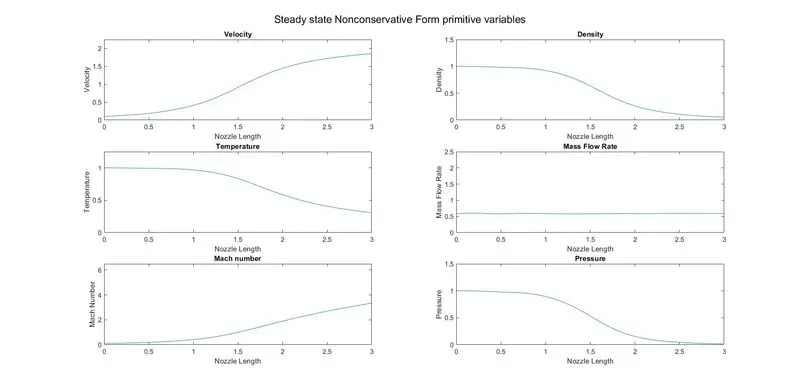
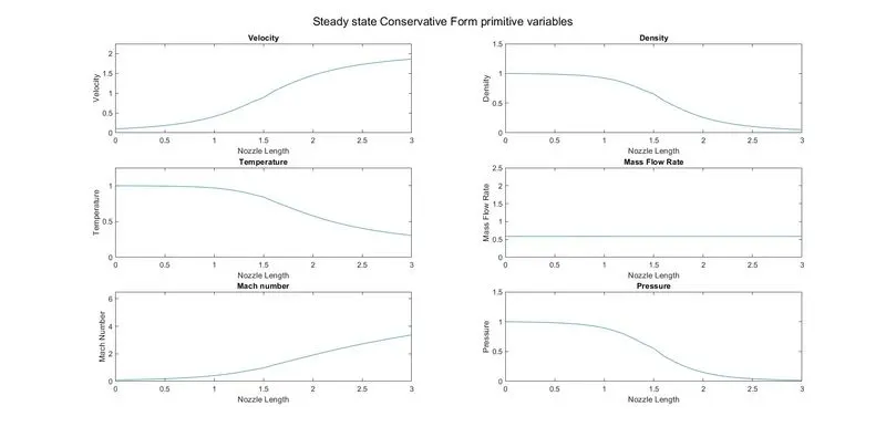
Observation:
The variation of the variables are plotted with nozzle length for both forms
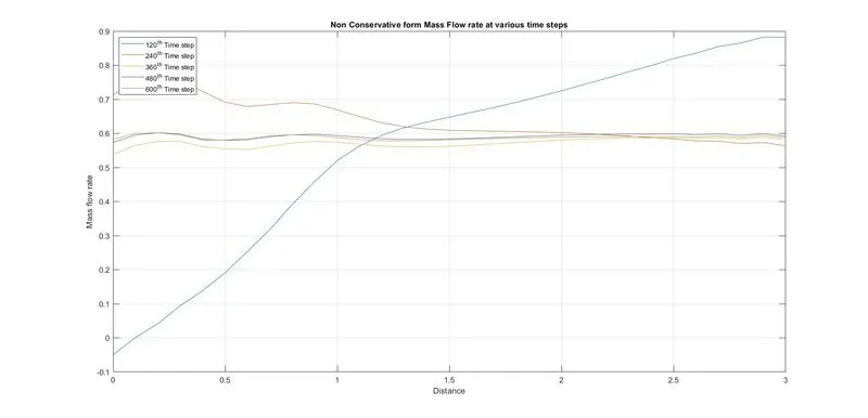
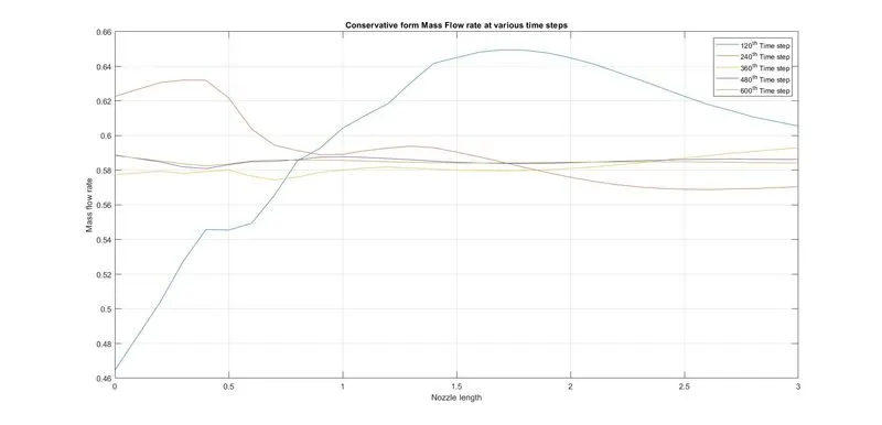
Observation:
The mass flow is steady at 400th time step in both forms
Comparision plot of Normalized mass flow rate of both Nonconservative and Conservative Forms:
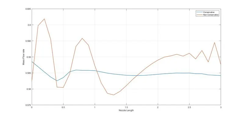
Observation:
The final solution varies similar to each form but the conservative solution is oscillating more than the nonconservative form. By this, we can understand that with a conservative approach the stability will acquire in a lesser number of iterations and time.
Grid Dependence Test:
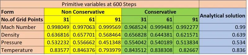
By comparing the grid points of 31,61 and 91 with the analytical solution we can conclude that if number of grid points increases the solution is more tend toward the correct solution.
So we can say that the problem is grid dependent.
Conclusion:
By calculating the values, there is enough evidence that the conservative form is more faster to calculate and more accurate to the desired solution. Though the accuracy is equal but the conservative form is more accurate.