Deriving 4th order approximation of a 2nd order derivative using Taylor Table method

function [y,am] = expr(x)

y = exp(x)*cos(x);
am = exp(x)* (-2*sin(x));

end

function error_c = central(x,dx,P,Q)

%N = number of Nodes
%P = order of accuracy
%Q = order of derivative

N = P+Q-1 ; %Number of nodes
k = (N-1)/2; %constant

A_c = zeros(N); %Defining matrix
B_c = zeros(N,1); %Defining matrix
B_c(Q+1,1) = 1; %Equating the constants on both sides

%Creating the coefficient matrix
for i = 1:N
    for j = 1 : N
        A_c(i,j) = ((-k+(j-1))^(i-1))/(factorial(i-1));
    end
end

[y,am] = expr(x); %Solving the expression
cons_c = (A_c^-1)*B_c; %Finding the coefficients
%Numerical Central method solution
d2f_c = ((cons_c(1)*expr(x-(2*dx))) + (cons_c(2)*expr(x-(1*dx))) + (cons_c(3)*expr(x+(0*dx))) + (cons_c(4)*expr(x+(1*dx))) + (cons_c(5)*expr(x+(2*dx))))/(dx^2);
error_c  = abs(am - d2f_c); %Error between central and analytical method

end

function error_sr = skewed_right(x,dx,P,Q)

%N = number of Nodes
%P = order of accuracy
%Q = order of derivative

N = P+Q ; %Number of nodes

A_sr = zeros(N); %Defining matrix
B_sr = zeros(N,1); %Defining matrix 
B_sr(Q+1,1) = 1; %Equating the constants on both sides

%Creating the coefficient Matrix
for i = 1:N
    for j = 1:N
        A_sr(i,j) = ((j-1)^(i-1))/(factorial(i-1));
    end
end

[y,am] = expr(x); %Solving the expression

cons_sr = (A_sr^-1)*B_sr; %finding the coefficients
%Numerical Skewed right difference scheme 
d2f_sr = ((cons_sr(6)*expr(x+(5*dx))) + (cons_sr(5)*expr(x+(4*dx))) + (cons_sr(4)*expr(x+(3*dx))) + (cons_sr(3)*expr(x+(2*dx))) + (cons_sr(2)*expr(x+(1*dx))) + (cons_sr(1)*expr(x+(0*dx))))/(dx^2);
error_sr = abs(am - d2f_sr); %Error between skewed right and analytical solution
end

function error_sl = skewed_left(x,dx,P,Q)

%N = number of Nodes
%P = order of accuracy
%Q = order of derivative

N = P+Q ; %Number of nodes

A_sl = zeros(N); %Defining matrix
B_sl = zeros(N,1); %Defining matrix
B_sl(Q+1,1) = 1; %Equating the constants on both sides

%Creating the coefficient matrix
for i = 1:N
    for j = 1:N
        A_sl(i,j) = ((-1)^(i+1))*((N-j)^(i-1))/(factorial(i-1));
    end
end

[y,am] = expr(x); %Solving the expression

cons_sl = (A_sl^-1)*B_sl; %Finding the coefficients
%Numerical Skewed left difference scheme
d2f_sl = ((cons_sl(1)*expr(x-(5*dx))) + (cons_sl(2)*expr(x-(4*dx))) + (cons_sl(3)*expr(x-(3*dx))) + (cons_sl(4)*expr(x-(2*dx))) + (cons_sl(5)*expr(x-(1*dx))) + (cons_sl(6)*expr(x+(0*dx))))/(dx^2);
error_sl = abs(am - d2f_sl); %Error between skewed left and analytical method
end

clear all
close all
clc

P = 4; %P = order of accuracy
Q = 2; %Q = order of derivative
x = pi/3; %Function at x
dx = linspace(1,0.01,500); %difference

for i = 1:length(dx)

    error_c(i) = central(x,dx(i),P,Q); %function to solve central  difference scheme
    error_sr(i) = skewed_right(x,dx(i),P,Q); %function to solve Skewed Right difference scheme
    error_sl(i) = skewed_left(x,dx(i),P,Q); %function to solve Skewed left difference scheme

end

loglog(dx,error_c,".-",dx,error_sl,".-",dx,error_sr,".-") %log log plot
legend({'Central','Skewed Left','Skewed Right'},'Location','northwest') % Legend
grid on

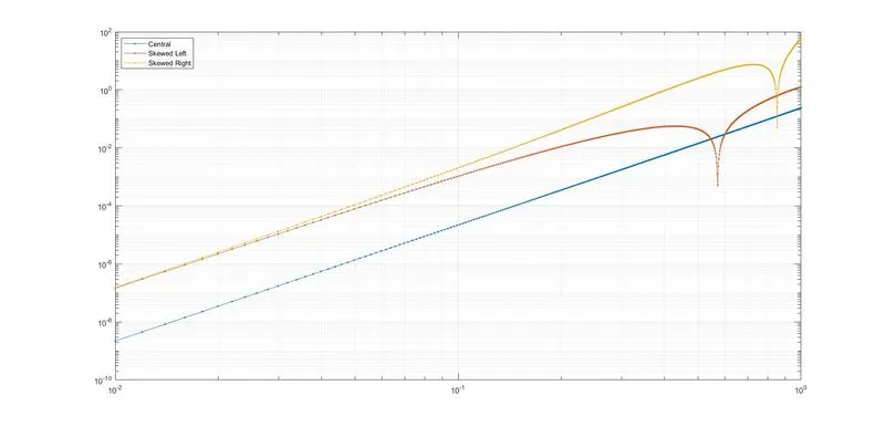
The first code contains the function of expression and the second derivative expression

Second, third and fourth functions "central", "skewed_right", and "skewed_left" derive the error between the analytical and numerical method scheme. As the above functions derive the matrix for the coefficients and solve the solution for fourth-order approximation of the second order.

The graph is plotted in log-log scale for the difference in 1 to 0.01 for 500 values.

The skewed scheme utilizes either point from left or right only to calculate the current point whereas the central uses both sides of the point. So, to calculate for the flow it uses the previous point to calculate that point as it is more accurate than the central scheme