Project 1 - Parsing NASA thermodynamic data

Aim:

To write a code in MATLAB to extract thermodynamic data from the file and calculate the cp, H and S for the species provided in the file and specified species.

Plot the thermodynamic properties with respect to the temperature in the respective folder which should be generated automatically.

Objective:

1. To write a function that extracts the 14 coefficients and calculates the enthalpy, entropy, and specific heats for all the species in the NASA thermodynamic data file "Thermo.dat".

The NASA polynomials have the form as shown below:

Where R is the universal gas constant, T is the temperature

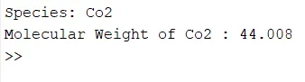
2. To calculate the molecular weight of each species and display it in the command window.

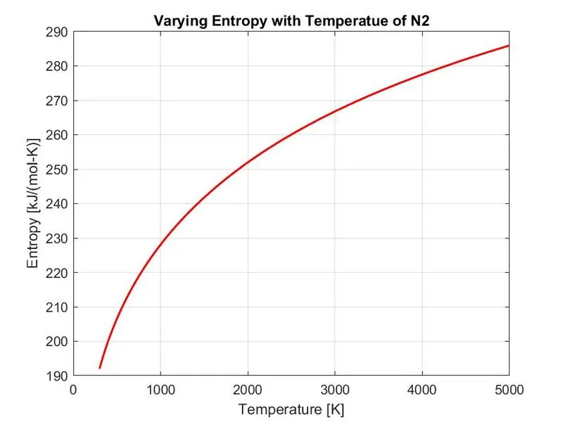
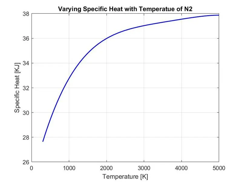
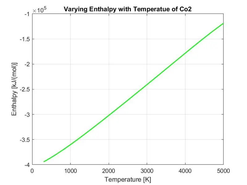
3. To plot the Cp, Enthalpy, and Entropy for the local temperature range (low temperature: high temperature) specific for each species.

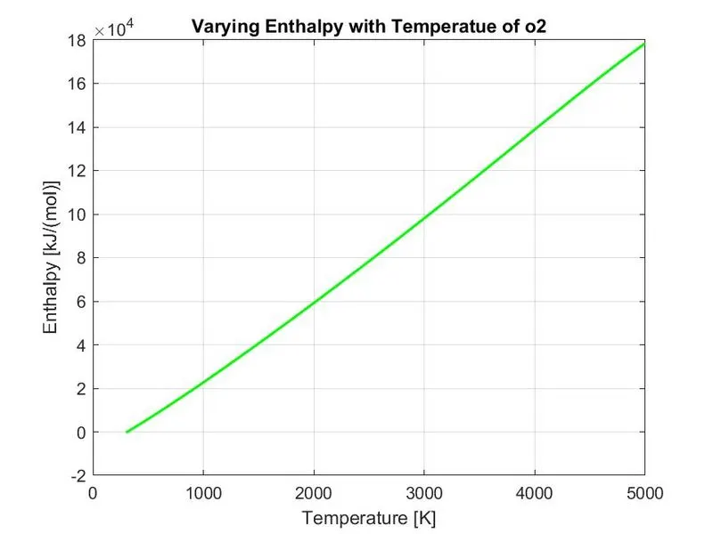
4. To save the plots as images with appropriate names and dump them in separate folders for each species with suitable name automatically.

Coefficient Function:

This function will result in the coefficients of all the species by using 'fgetl' line command to read every line of the file. First, it will calculate the global temperatures from the file.

Then the code will run 'fgetl' function 212 times to store the 14 coefficients the lines are read by multiples of 1, 2, 3 and 4 respectively to store the coefficients at each line. To obtain the temperature range from the Thermo.dat file, using ‘strsplit’ to split the temperature into a particular string cell. Used ‘str2num’ for converting string cell to numbers.

%Coeffiecint Function

function [global_low_temp,global_mid_temp,global_high_temp,Species,a1,a2,a3,a4,a5,a6,a7,a8,a9,a10,a11,a12,a13,a14] = coefficients()
    
    file = fopen("THERMO.dat",'r');         %File parasing
    get = fgetl(file);                      %Reading file line
    
    global_temp = fgetl(file);                              %Global temperatures
    global_temp_split= strsplit(global_temp," ");
    global_low_temp  = str2double(global_temp_split{2});
    global_mid_temp  = str2double(global_temp_split{3});
    global_high_temp = str2double(global_temp_split{4});
    
    for i = 1:3
        get = fgetl(file);
    end

    n_1 = 1;
    n_2 = 1;
    n_3 = 1;
    n_4 = 1;
    
    for i = 1:212
    
        get = fgetl(file);
    
        k_1 = (1:4:212);
        k_2 = (2:4:212);
        k_3 = (3:4:212);
        k_4 = (4:4:212);
    
        p_1 = ismember(i,k_1);                      %Checking the lines
        p_2 = ismember(i,k_2);
        p_3 = ismember(i,k_3);
        p_4 = ismember(i,k_4);
    
        if p_1 == 1                                 %Species identification
            H = strsplit(get,' ');
            Species(n_1) = {(H{1})};
            n_1 = n_1+1;
        end
    
        if p_2 == 1                                 %Coefficient identification
            q = strfind(get,'E');
            a1(n_2) = str2double(get(1:q(1)+3));
            a2(n_2) = str2double(get(q(1)+4:q(2)+3));
            a3(n_2) = str2double(get(q(2)+4:q(3)+3));
            a4(n_2) = str2double(get(q(3)+4:q(4)+3));
            a5(n_2) = str2double(get(q(4)+4:q(5)+3));
            n_2 = n_2+1;
        end
    
        if p_3 == 1
            q = strfind(get,'E');
            a6(n_3) = str2double(get(1:q(1)+3));
            a7(n_3) = str2double(get(q(1)+4:q(2)+3));
            a8(n_3) = str2double(get(q(2)+4:q(3)+3));
            a9(n_3) = str2double(get(q(3)+4:q(4)+3));
            a10(n_3) = str2double(get(q(4)+4:q(5)+3));
            n_3 = n_3+1;
        end
    
        if p_4 == 1
            q = strfind(get,'E');
            a11(n_4) = str2double(get(1:q(1)+3));
            a12(n_4) = str2double(get(q(1)+4:q(2)+3));
            a13(n_4) = str2double(get(q(2)+4:q(3)+3));
            a14(n_4) = str2double(get(q(3)+4:q(4)+3));
            n_4 = n_4+1;
         end
            
         
    end

    Species = string(Species);
    fclose(file);                                   %Closing file

end

Molecular Weight Function:

This function will take Species as the input to find the molecular weight and display the molecular weight in the command window.

%Moecular weight function

function m_w = molecular_weight(Species)

    sp = char(Species);   %Converting to character
    m_w = 0;
    
    atomic_name = ['H','C','O','N','A'];                %Atomic names
    atomic_weight = [1.00784,12.0096,15.99903,14.00643,39.948];     %Atomic weights
    
    for i = 1:strlength(Species)                    %Nested loop for each char in species
        for j = 1:length(atomic_name)
            if strcmpi(sp(i),atomic_name(j))
                m_w = m_w+atomic_weight(j);
                pos = j;
            end
        end
        n = str2double(sp(i));
        if n>1
            m_w = m_w + ((n-1)*atomic_weight(pos));
        end
    end
    
    fprintf('Molecular Weight of %s : %0.3f \n',Species,m_w);       %Print the molecular weight

end

Specific Heat Function:

This function will take coefficients as input and global temperature to calculate the cp.

%Specific heat function

function [cp] = specific_heat(a1,a2,a3,a4,a5,a8,a9,a10,a11,a12,T,R,global_mid_temp)

    if T <= global_mid_temp                                             %Calculating the cp with temperature
        cp = R.*(a8+(a9*T)+(a10*(T.^2))+(a11*(T.^3))+(a12*(T.^4)));
    else
        cp = R.*(a1+(a2.*T)+(a3.*(T.^2))+(a4.*(T.^3))+(a5.*(T.^4)));
    end

end

Entropy Function:

This function will take coefficients as input and global temperature to calculate the S.

%Entropy function

function [S] = entropy(a1,a2,a3,a4,a5,a7,a8,a9,a10,a11,a12,a14,T,R,global_mid_temp)

    if T <= global_mid_temp                                   %Calculating the S with temperature
        S = R.*((a8.*log(T))+ (a9.*T) + (a10*((T).^2)/2) + (a11*((T).^3)/3) + (a12*((T).^4)/4) + a14);
    else
        S = R.*((a1.*log(T)) + (a2.*T) + (a3*((T).^2)/2) + (a4*((T).^3)/3) + (a5*((T).^4)/4) + a7);
    end

end

Enthalpy Function:

This function will take coefficients as input and global temperature to calculate the H.

% Enthalpy Calculation function

function [H] = enthalpy(a1,a2,a3,a4,a5,a6,a8,a9,a10,a11,a12,a13,T,R,global_mid_temp)    
% Comparing with global Terature
% If less than global Terature - minimum coefficients are taken
 
    if T <= global_mid_temp
        H = R*T.*(a8 + ((a9*T)/2) + ((a10*(T).^2)/3) + ((a11*(T).^3)/4) + ((a12*(T).^4)/5) +((a13./T)));
    else          
        H = R*T.*(a1 + ((a2*T)/2) + ((a3*(T).^2)/3) + ((a4*(T).^3)/4) + ((a5*(T).^4)/5) +((a6./T)));
    end

end

Main:

This function will use the above functions to calculate the cp, S and H and will plot the data and save it in the respective folder.

clear all
close all
clc

%Coefficients are calculated
[global_low_temp,global_mid_temp,global_high_temp,Species,a1,a2,a3,a4,a5,a6,a7,a8,a9,a10,a11,a12,a13,a14] = coefficients();

%Temperature points
 T = linspace(global_low_temp,global_high_temp,1000);
 R = 8.314;

  for i = 1:length(Species)

      m_w = molecular_weight(Species(i));               %Molecular Weight
      file = fopen('Molecular_weight.txt','a+');        %Creating file
      fprintf(file,'Molecular Weight of %s is %0.3f \n',Species(i),m_w);
      fclose(file);
      [cp] = specific_heat(a1(i),a2(i),a3(i),a4(i),a5(i),a8(i),a9(i),a10(i),a11(i),a12(i),T,R,global_mid_temp);
      [S] = entropy(a1(i),a2(i),a3(i),a4(i),a5(i),a7(i),a8(i),a9(i),a10(i),a11(i),a12(i),a14(i),T,R,global_mid_temp);
      [H] = enthalpy(a1(i),a2(i),a3(i),a4(i),a5(i),a6(i),a8(i),a9(i),a10(i),a11(i),a12(i),a13(i),T,R,global_mid_temp);
        
      %Creating folder 
      cur_dir = pwd;
      mkdir(Species(i));
      cd(Species(i));
        
      %CP plot and image save
      a = figure('visible','off');
      plot(T,cp,'linewidth',1.5,'color','b');
      xlabel('Temperature [K]');
      ylabel('Specific Heat [KJ]');
      title(sprintf('Varying Specific Heat with Temperatue of %s',Species(i)));
      grid on
      saveas(a,'Specific Heat.jpg');

      %S plot and image save
      b = figure('visible','off');
      plot(T,S,'linewidth',1.5,'color','r');
      xlabel('Temperature [K]');
      ylabel('Entropy [kJ/(mol-K)]');
      title(sprintf('Varying Entropy with Temperatue of %s',Species(i)));
      grid on
      saveas(b,'Entropy.jpg');

      %H plot and image save
      c = figure('visible','off');
      plot(T,H,'linewidth',1.5,'color','g');
      xlabel('Temperature [K]');
      ylabel('Enthalpy [kJ/(mol)]');
      title(sprintf('Varying Enthalpy with Temperatue of %s',Species(i)));
      grid on
      saveas(c,'Enthalpy.jpg');      

      %Back to the primary folder
      cd(cur_dir);

  end

Individual Species Code:

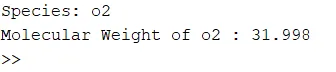
This will take the species as input and plot the graphs and creates the folder to store the graphs.

clear all
close all
clc

%Coefficients are calculated
[global_low_temp,global_mid_temp,global_high_temp,Species,a1,a2,a3,a4,a5,a6,a7,a8,a9,a10,a11,a12,a13,a14] = coefficients();

s = input('Species: ','s');

T = linspace(global_low_temp,global_high_temp,1000);
R = 8.314;

%Finding the coefficient array in the database
k = strcmpi(s,Species);
i = find(k==1);

m_w = molecular_weight(s);
cp = specific_heat(a1(i),a2(i),a3(i),a4(i),a5(i),a8(i),a9(i),a10(i),a11(i),a12(i),T,R,global_mid_temp);
S = entropy(a1(i),a2(i),a3(i),a4(i),a5(i),a7(i),a8(i),a9(i),a10(i),a11(i),a12(i),a14(i),T,R,global_mid_temp);
H = enthalpy(a1(i),a2(i),a3(i),a4(i),a5(i),a6(i),a8(i),a9(i),a10(i),a11(i),a12(i),a13(i),T,R,global_mid_temp);

cur_dir = pwd;
mkdir(s);
cd(s);

%CP plot and image save
a = figure('visible','off');
plot(T,cp,'linewidth',1.5,'color','b');
xlabel('Temperature [K]');
ylabel('Specific Heat [KJ]');
title(sprintf('Varying Specific Heat with Temperatue of %s',s));
grid on
saveas(a,'Specific Heat.jpg');

%S plot and image save
b = figure('visible','off');
plot(T,S,'linewidth',1.5,'color','r');
xlabel('Temperature [K]');
ylabel('Entropy [kJ/(mol-K)]');
title(sprintf('Varying Entropy with Temperatue of %s',s));
grid on
saveas(b,'Entropy.jpg');

%H plot and image save
c = figure('visible','off');
plot(T,H,'linewidth',1.5,'color','g');
xlabel('Temperature [K]');
ylabel('Enthalpy [kJ/(mol)]');
title(sprintf('Varying Enthalpy with Temperatue of %s',s));
grid on
saveas(c,'Enthalpy.jpg');

cd(cur_dir);

Result:

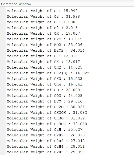
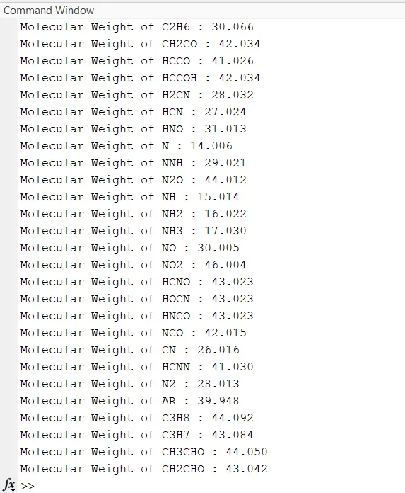
o2:

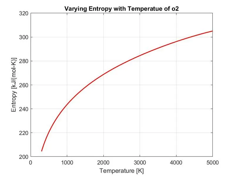
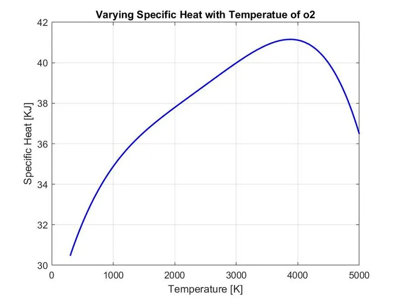
N2:

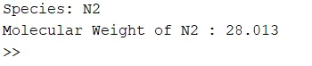
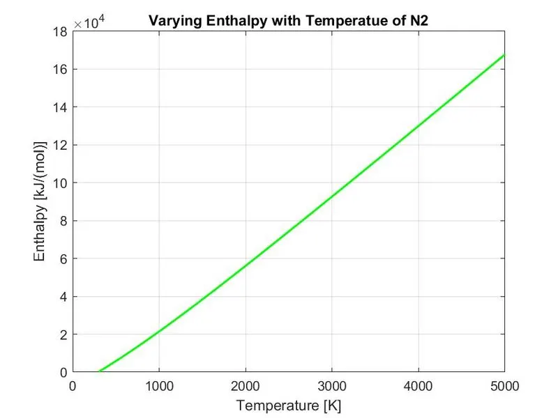
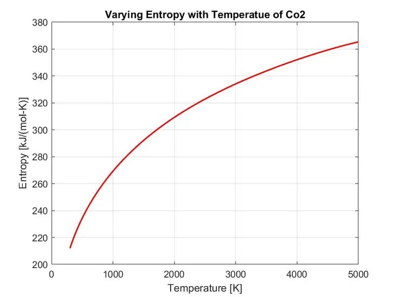
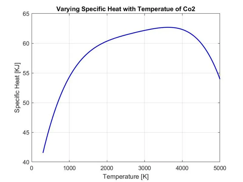
Co2:

Conclusion :

Using MATLAB code, the necessary coefficients required to evaluate various thermodynamic parameters for different species are extracted from NASA thermodynamic data file. The specific heat, enthalpy, and entropy for all the species are calculated and plotted against the local temperature range. The molecular weight is calculated for all the species.