Week 2 - Flow over a Cylinder.
In this project, a basic two-dimensional flow over a cylinder will be conducted for a wide range of reynold's numbers. A cylinder is a basic geometric shape that is seen everywhere, and there are multiple literatures that confirm an unstable region behind the cylinder beyond a certain reynold's number.
This instablity gives rise to a surprising periodic phenomenon called the Von Karman vortex street, which only occurs at low reynold's numbers. It is a repeating pattern of swirling vortices, caused by a process known as vortex shedding, which is responsible for the unsteady separation of flow of a fluid around blunt bodies. This is the phenomenon responsible for the apparent "singing" of telephone lines and it only happens within a range of reynold's numbers. Typically above 90.
This project will be divided into two major parts, each part will be divided by a number of sub-parts.
Part 1
For Re = 100, simulating flow over cylinder for both steady and transient cases
Part 2
For Re = 10, 100, 1000, 10000 and 100000, simulating flow over cylinder with the steady state solver and compare drag coefficient data with empirical data.
The geometry, mesh and most of the solution setup is the same for all parts and sub-parts.
Geometry
The geometry of this project is quite simple and can be made in spaceclaim. The diameter of the cylinder (D) is used as the standard measurement for other dimensions of the geometry.
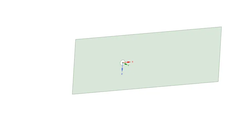
The geometry consists of a circle with diameter (D) centered around the origin on the XZ plane. The circle is surrounded by a rectangular wind tunnel lying on the same plane. The left edge of the rectangle (inlet) is 10*D the distance from the origin, the outlet is 20*D from the origin, and the height of the rectangle is 10*D centered about the Y axis. The sketch lines are converted into a surface and the geometry is ready for meshing. The diameter for this project is 2 meters.
This is the finished geometry seen in spaceclaim:
Meshing
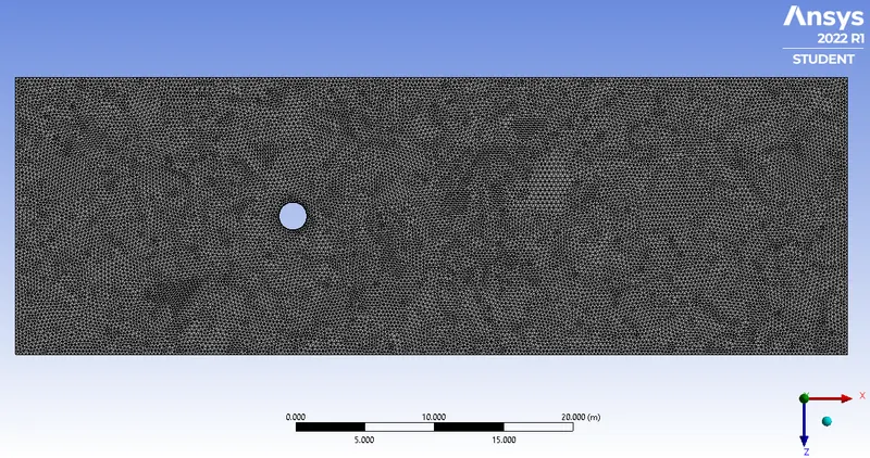
The mesh size used was 0.25m.
Additional Mesh controls were used to modify the mesh. They are as follows:
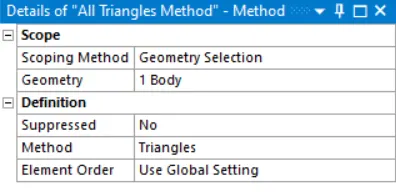
1. Method -> Triangles: The originally generated mesh was made of quad elements which are less desirable for this solution. Triangle elements were selected.
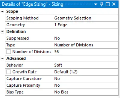
2. Edge Sizing -> Number of Divisions: The number of cells around the cylinder was very low which will lead to poor results near the cylindrical wall. The wall/cylinder edge was smoothed out using this tool to 36 edges for the wall.
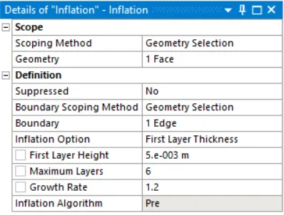
3. Inflation -> First Layer Thickness: This method was used to enhance the cell count in the regions near the wall, to increase solution accuracy.
This is the resultant mesh seen in ANSYS:
Mesh Quality
The quality of the mesh can be seen using the mesh metrics tab:

Most elements have a score of >0.7, hence the mesh can be considered satisfactory.
Setup
Boundaries
inlet - inlet
outlet - pressure outlet
walls - wall (no-slip)
top and bottom - symmetry
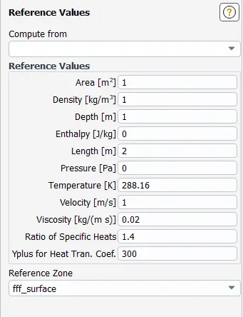
Reference Values
The most important values here are: Area, Density, Length and Velocity.
Materials
The existing material (air) was removed and a new material was created
We know, Reynold's Number
`Re = (rho * u * D)/mu`
For all simulations: density (`rho`) and inlet velocity (`u`) were kept constant. Hence, the reynold's number's variation was only made through changing the kinematic viscosity (`mu`).
`D = 2m, u = 1 m//s and rho = 1`
`Re = (1*1*2)/mu`
`=> Re = 2/mu`
Viscous
Laminar was used for some simulations, k-omega SST for others.
Reports
Three reports were created.
1. Lift Coefficient of wall
2. Drag Coefficient of wall
3. Velocity monitor at a point - a point was manually created at x = 4, y = 0 to observe vortex velocity
Solution - Methods
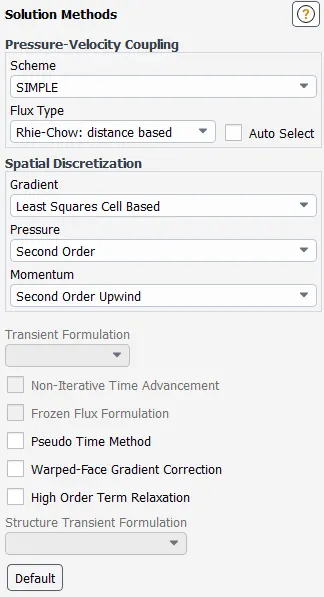
This is very important else the solution will not be correct.
Part 1
Steady State Solver
Solver: Steady State Solver
Kinematic Viscosity of fluid (kg/m.s): 0.02
Reynold's Number: 100
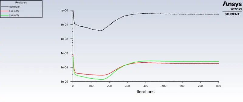
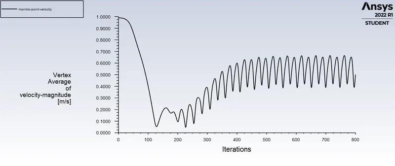
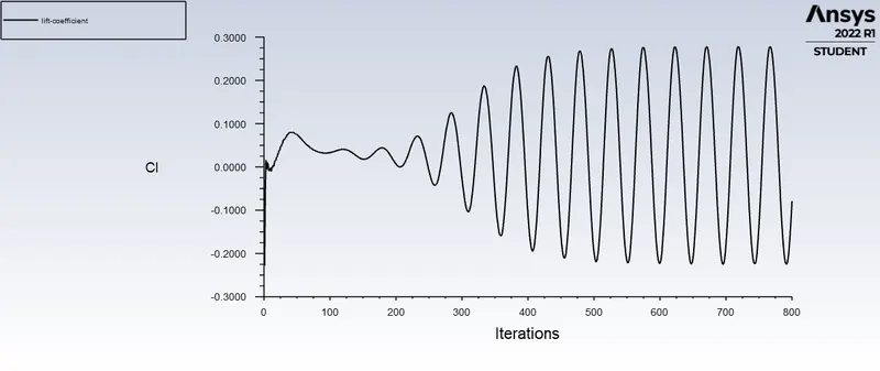
The solution is converged even though residuals aren't low enough because of the observed periodicity of monitor point's velocity. Even if the simulation is ran for another 1000 iterations, the residuals would not decrease. The periodicity is because of the vor karman vortex street.
Residuals
Velocity at monitor point
Lift coefficient
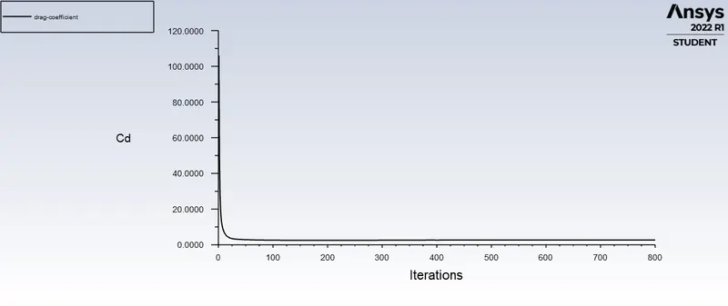
Drag coefficient
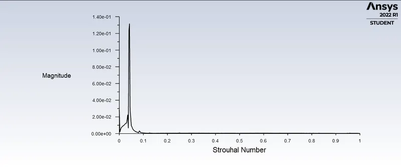
In order to calculate the periodicity of the lift coefficient, an FFT (fast fourier transform) was conducted to find the Strouhal number for this case. It was calculated using ANSYS's FFT tool with the following settings:
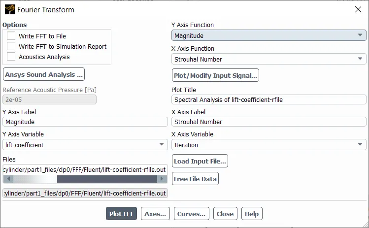
Strouhal number
Transient Solver
Since the steady state solver is quite inaccurate when it comes to intermediate values, because the main goal of a steady state simulation is to capture the
Solver: Transient Solver
Kinematic Viscosity of fluid (kg/m.s): 0.02
Reynold's Number: 100
Timesteps: 600
Stepsize: 0.1s
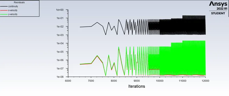
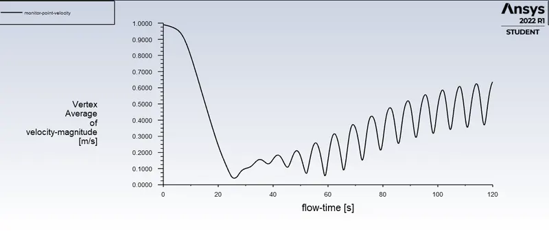
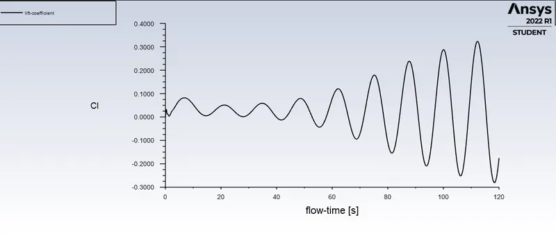
The solution is converged even though residuals aren't low enough because of the observed periodicity of monitor point's velocity. Even if the simulation is ran for another 1000 iterations, the residuals would not decrease. The periodicity is because of the vor karman vortex street.
Residuals
Velocity at monitor point
Lift coefficient
Drag coefficient
In order to calculate the periodicity of the lift coefficient, an FFT (fast fourier transform) was conducted to find the Strouhal number for this case. It was calculated using ANSYS's FFT tool with the following settings:
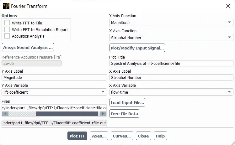
Strouhal number
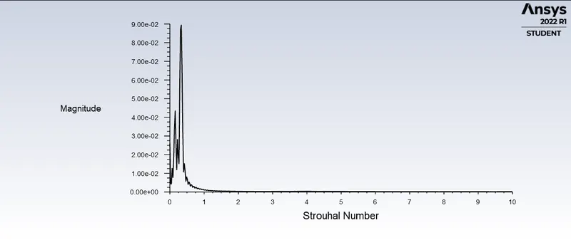
Part 2
All simulations in this part are done using the steady state solver, the kinematic viscosity is varied to change the reynold's number.
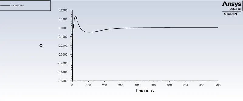
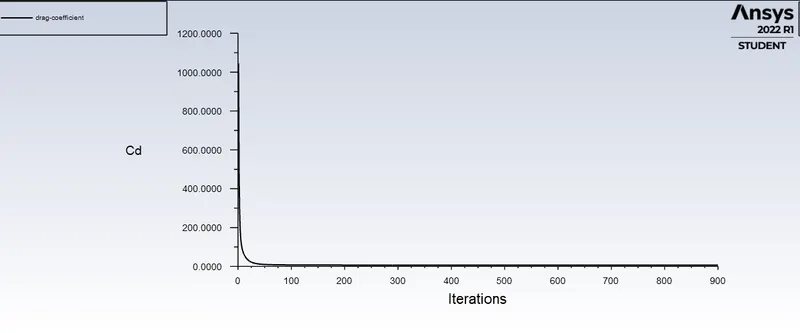
Reynold's Number: 10
Kinematic Viscosity of fluid (kg/m.s): 0.2
The solution is said to be converged because of the low value of the residuals and the stable value of velocity at the monitor point.
Residuals
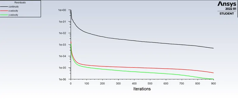
Velocity at monitor point
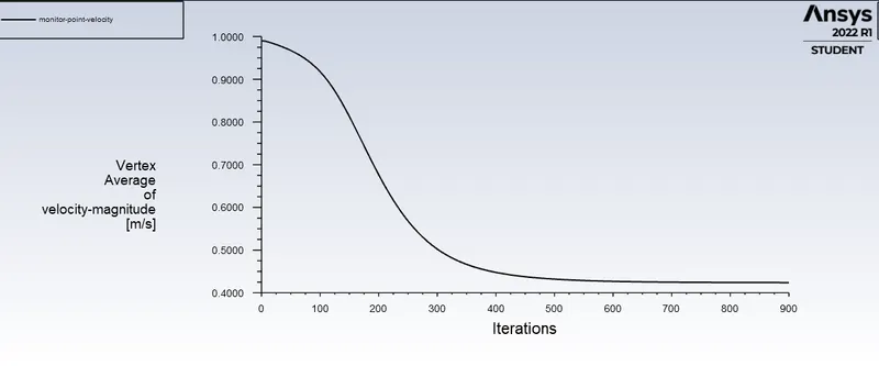
Lift Coefficient
Drag Coefficient
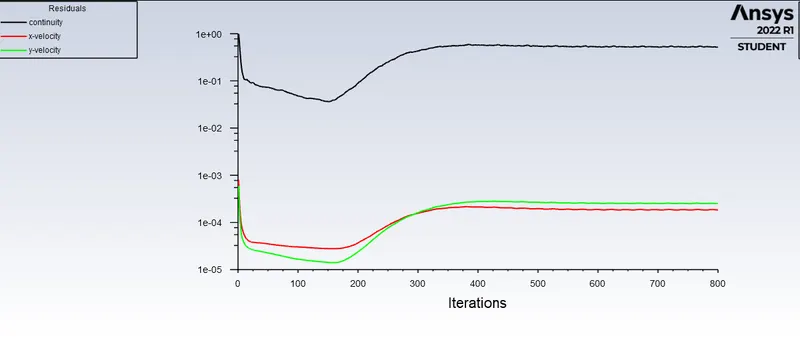
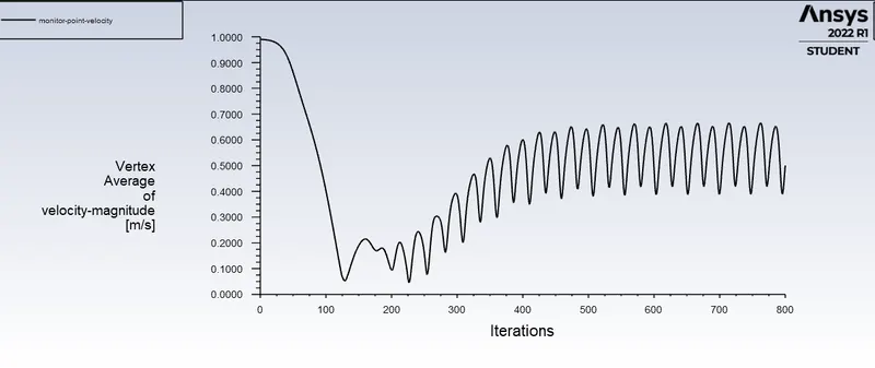
Reynold's Number: 100
Kinematic Viscosity of fluid (kg/m.s): 0.02
The solution is said to be converged because of the low value of the residuals and the stable value of velocity at the monitor point.
Residuals
Velocity at monitor point
Lift Coefficient
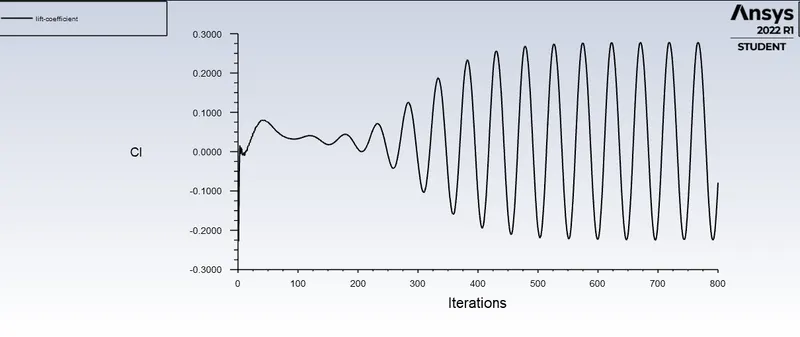
Drag Coefficient
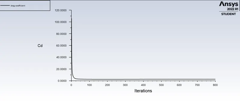
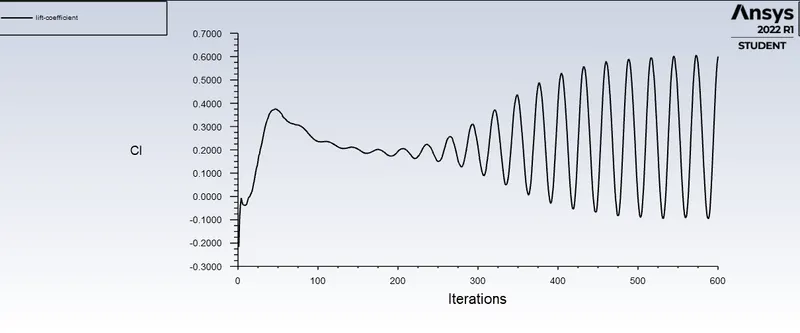
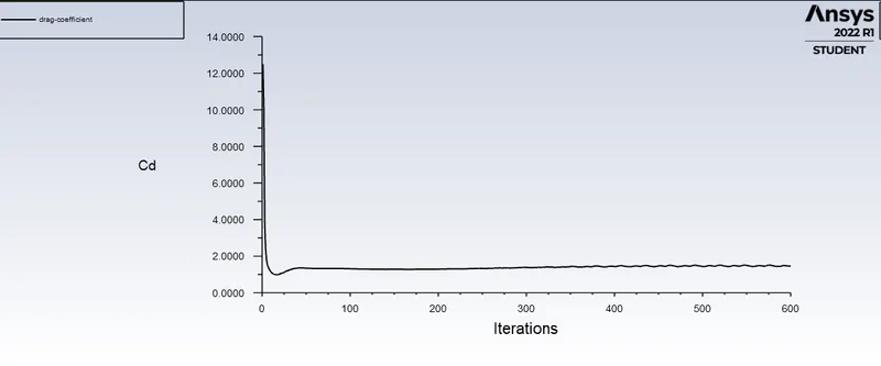
Reynold's Number: 1000
Kinematic Viscosity of fluid (kg/m.s): 0.002
Since flow will become turbulent behind the cylinder in this case, so viscous model was switched to k-omega SST.
The solution is said to be converged because of the low value of the residuals and the stable value of velocity at the monitor point.
Residuals
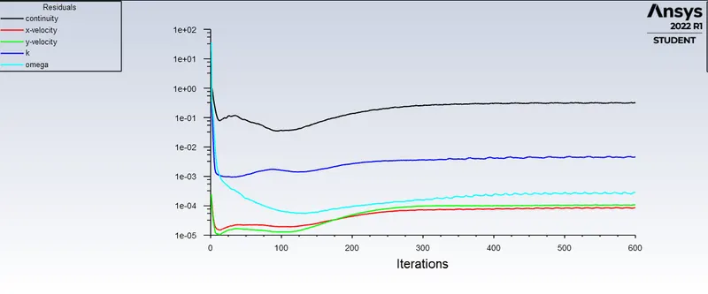
Velocity at monitor point
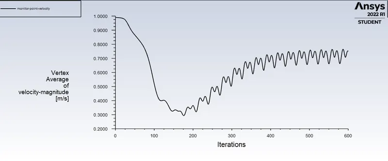
Lift Coefficient
Drag Coefficient
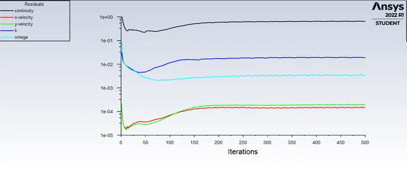
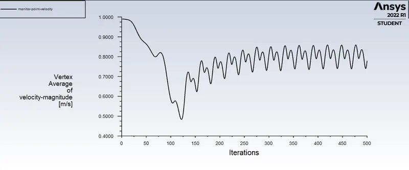
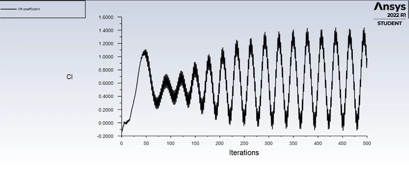
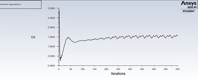
Reynold's Number: 10000
Kinematic Viscosity of fluid (kg/m.s): 0.0002
Since flow is turbulent in this case, so viscous model was switched to k-omega SST.
The solution is said to be converged because of the observed periodicity of velocity at the monitor point.
Residuals
Velocity at monitor point
Lift Coefficient
Drag Coefficient
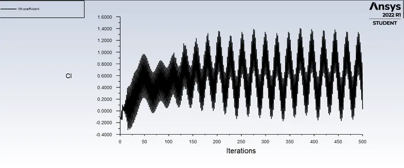
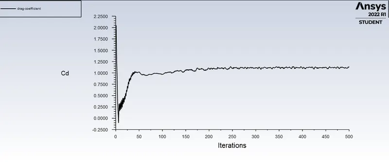
Reynold's Number: 100000
Kinematic Viscosity of fluid (kg/m.s): 0.00002
Since flow is turbulent in this case, so viscous model was switched to k-omega SST.
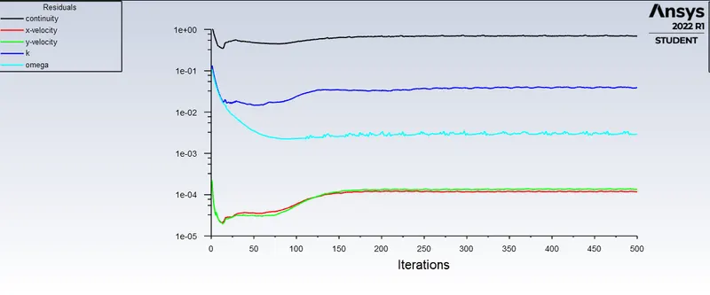
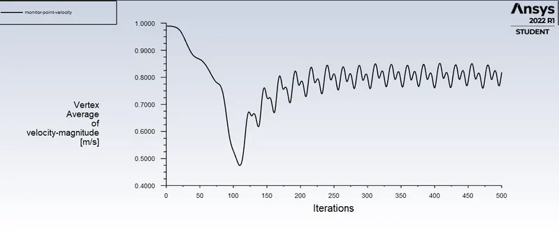
The solution is said to be converged because of the observed periodicity of velocity at the monitor point.
Residuals
Velocity at monitor point
Lift Coefficient
Drag Coefficient
Comparison between experimental and simulation data
The coefficient of drag of the cylinder is compared between experimental and simulation data.
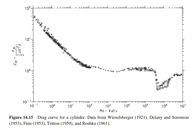
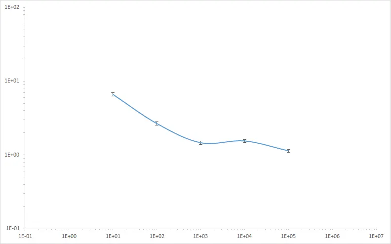
The scales are same for both plots for easy viewing.
After superimposing both plots,
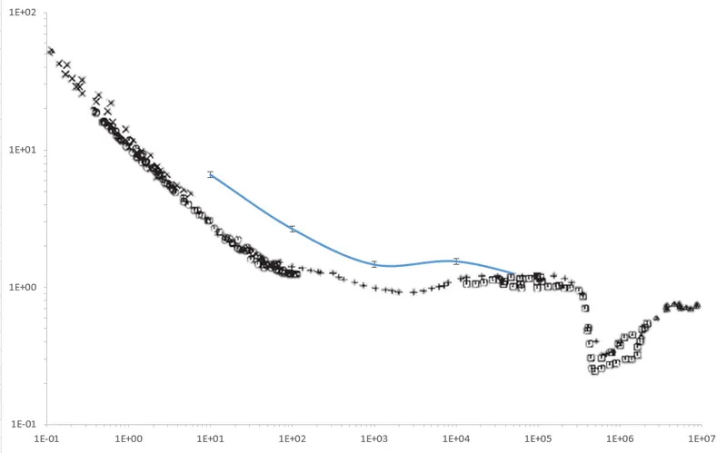
The simulation data agrees with experimental data to a certain extent, the general trends are visible.
Animation
This is the animation for part 1's transient simulation, as transient simulations are the most accurate for values during the simulation.
Conclusions and Observations
- Steady State simulation is less accurate than transient, but steady state is solved more faster than a transient simulation.
- Von karman vortex street is only occurs at around Re = 100, and not at other ranges. This is as expected from empirical evidence.
- Beyond Re = 100, flow becomes turbulent among the edges of the cylinder. Beyond Re = 1000, turbulent flow is everywhere.
- Beyond a critical reynold's number, the flow is too fluidic to cause any vortices or periodic motion.
- The von karman vortex sheet has a periodic pattern and it can be quantified using the Strouhal number.
- The simulation data and experimental data agree to a certain extent. To increase the accuracy of simulation data, further mesh refinement is required
- Vortices which are formed beyond a certain reynold's number will be visible if mesh resolution is increased in that area.
References
1. 14.6 FLOW AROUND A CIRCULAR CYLINDER, Incompressible Flow, Fourth Edition Ronald L. Panton
2. Numerical simulation of laminar flow past a circular cylinder, B.N. Rajani, A. Kandasamy, Sekhar Majumdar.
3. https://cfdflowengineering.com/cfd-modeling-of-flow-over-a-cylinder/