Week 4.1 - Solving second order ODEs

The second order differential equation has been converted into a set of two first order differential equations, which can be solved in MATLAB easily.

The conditions of the simulation are as follows:

L = 1 `m`, m = 1 kg, b = 0.05 `Ns//m`, g = 9.81 `m//s^2`.

The intial conditions are as follows:

Angular displacement = 0 `rad`, angular velocity = 0.5 `rad//s`. (Note: angular velocity of 3 `rad//s` meant that the pendulum did multiple full revolutions around the center.

Code (with explanation)

Function

The purpose of this function is to solve the set of ODEs and return the solution. The input paramets are the time span and initial conditions while the angular displacement and angular velocity of the pendulum are the output parameters.

filename: ode_pendulum.m

% purpose of this function is to solve the set of ODEs and return the solution

function [thetadot] = ode_pendulum (t, theta)

    % initialising input values
    b = 0.05;
    m = 1;
    l = 1;
    g = 9.81;
    
    thetadot = zeros (2,1); 
    
    thetadot(1) = theta(2);  % equation 1
    
    thetadot(2) = (-1*(b*theta(2)/m)-(g*sind(theta(1))/l)); % equation 2

end

Main Program

The main program will call the function, and receive the solution. The received solution will be plotted and the animation will be generated as well.

clear all
close all
clc

% initialising input values
b = 0.05; % damping coefficient (Ns/m)
m = 1;    % mass of pendulum's ball (kg)
l = 0.2;  % length of string of pendulum (m)
g = 9.81; % gravitational acceleration (m/s^2)

% the timespan/time period of oscillation
t = linspace(0,20,100);

% initial conditions. initial angular displacement is 0 rad and initial angular
% velocity is 0.5 rad/s
theta0 = [0;0.5];

% ode function time period in theta1, ode45 solves for displacement and velocity
% in theta(:,1) and theta (:,2) respectively
[t ,theta] = ode45('ode_pendulum', t, theta0);

ct = 1; % counter varaible for animation frames

% for loop to generate animation of the pendulum
for i=1:length(theta)

    x=l*sin(theta(i,1));  
    y=-1*l*cos(theta(i,1));  % calculating coordinates of center of pendulum ball

    plot([-0.1 0 0.1],zeros(1,3),'linewidth',3) % plotting horizontal line
    hold on
    plot(linspace(x,0,5) ,linspace(y,0,5),'color','bla') % plotting string of pendulum
    hold on
    plot(x,y,'o','markersize',20,'color','r') % plotting the pendulum
    hold on
    axis([-0.25 0.25 -0.3 0.1]) % making the pendulum centered in the animation
    axis off % removing uneseccary clutter
    M(ct)=getframe(gcf); % storing each frame in structure M
    ct = ct + 1;
    clf 
end  

close all
% converting frames into a video
videofile=VideoWriter('test.avi','Uncompressed AVI');
open (videofile);
writeVideo (videofile,M);
close(videofile);

% figure showing plot of time vs angular displacement

figure (2)
plot(t,theta(:,1),'color','r','linewidth',1) 
xlabel('Time (s)')
ylabel('Angular Displacement (rad)')

% figure showing plot of time vs angular velocity

figure (3)
plot(t,theta(:,2),'color','b','linewidth',1)
xlabel('Time (s)')
ylabel('Angular Velocity (rad/s)')

Output

Angular Displacement vs Time

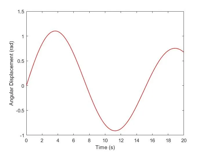
Graph of angular displacement vs time is generated, the displacement eventually tends to zero due to damping but this is not visible due to limited simulation time.

Angular Velocity vs Time

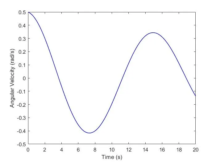
Graph of angular velocity vs time is generated, the velocity eventually tends to zero due to damping but this is not visible in this graph due to limited simulation time.

Animation of Pendulum

https://youtu.be/HOCVqsgXsg0

Errors Faced

The function ode_pendulum couldn't take more than two input parameters.

Command Window Screenshot

Solution to the Error

Instead of passing b, g, m and l as parameters, they were defined in the function.