Week 1: Channel flow simulation using CONVERGE CFD
Aim:
1. To setting up a channel flow tutorial by using the converge.
2. To run the case for three different base mesh sizes by Cygwin
3. To post process using the Paraview
4. To compare the results between all the simulation
Geometry
Mesh Size
dx = 2e-4m, dy = 2e-4m, dz = 2e-4m
dx = 1.5e-4m, dy = 1.5e-4m, dz = 1.5e-4m
dx = 1.0e-4m, dy = 1.0e-4m, dz = 1.0e-4m (If this is too much for your PC, use 1.2e-4m)
Geometry/Model
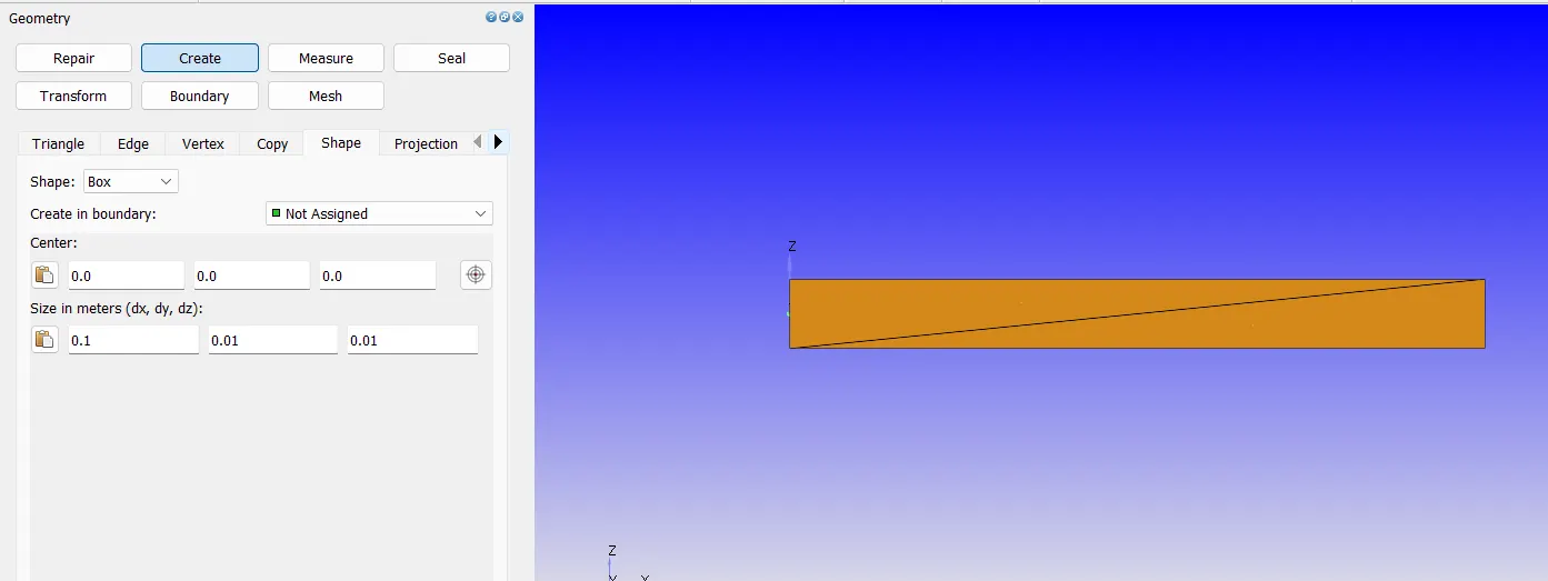
Create the Channel using geometry option, selected the Box in shape option. Given the dimension. Then applied.
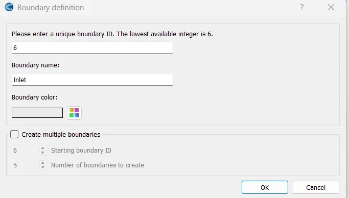
To create the boundaries, select the
boundary tab , Create new boundary by using the” +” icon. Define the ID , Name and color of the
surface. Then ok
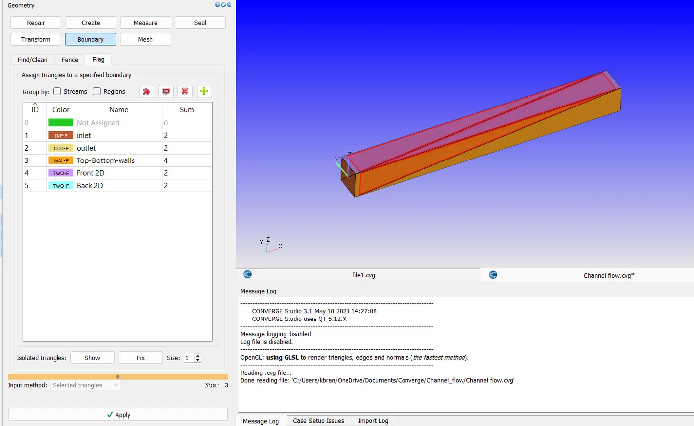
Select the surface in the model, and the select the boundary, then apply and we can observe that surface color will change according to Boundary ID and name.
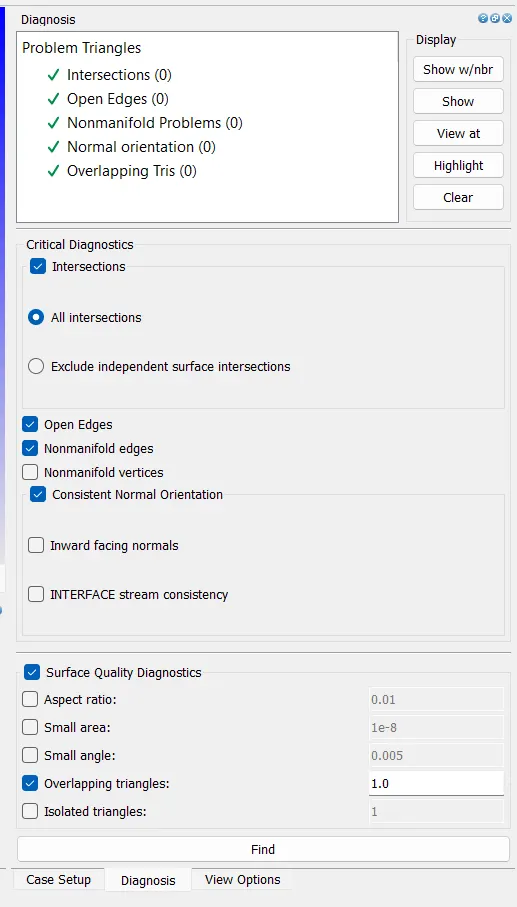
After assign the boundary, Diagnosis the geometry by diagnosis option,
Case setup
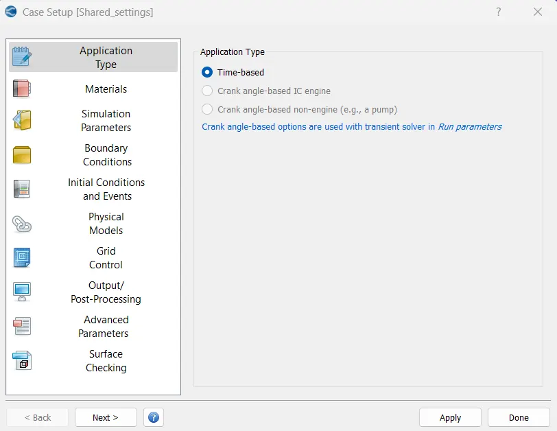
Time based simulation has been selected for the simulation
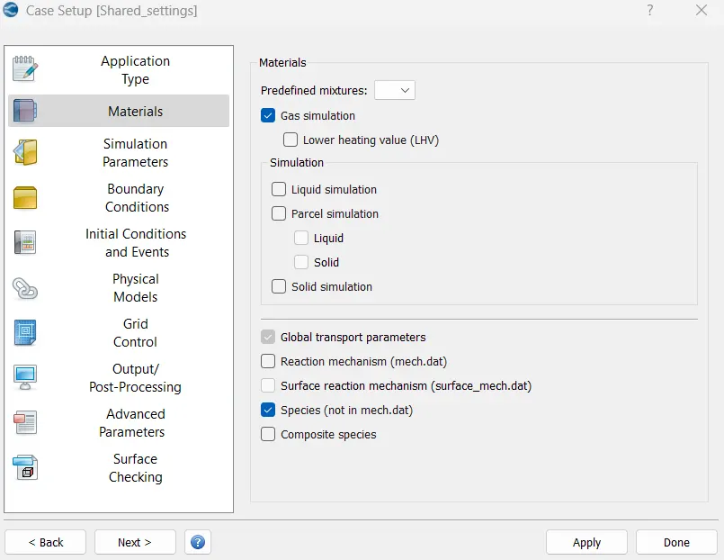
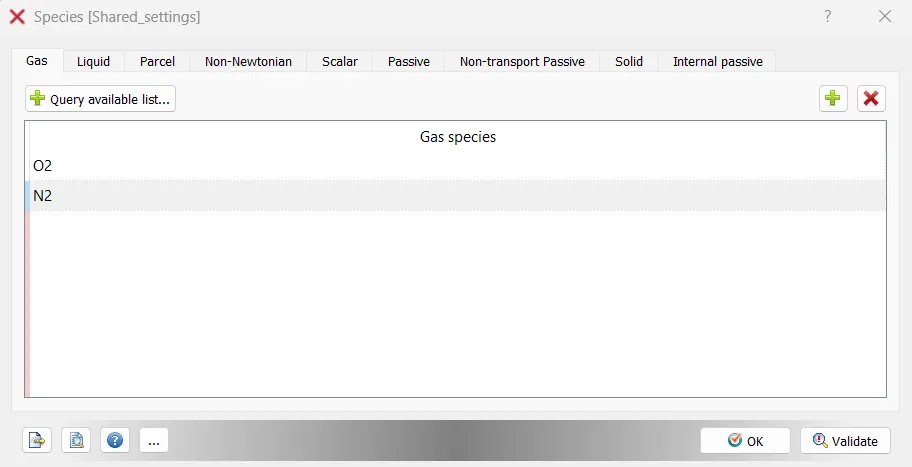
Gas Simulation
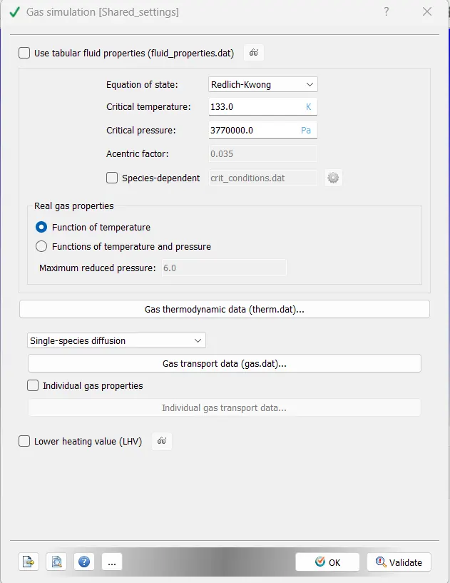
Global transport Parameters
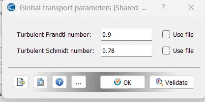
Species
Simulation Parameters,
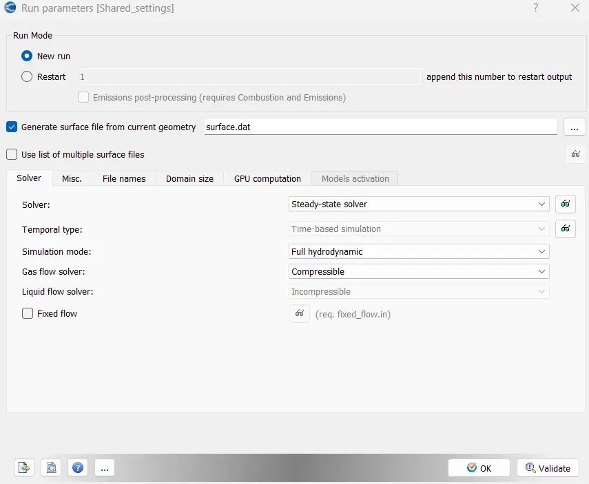
Run Parameter
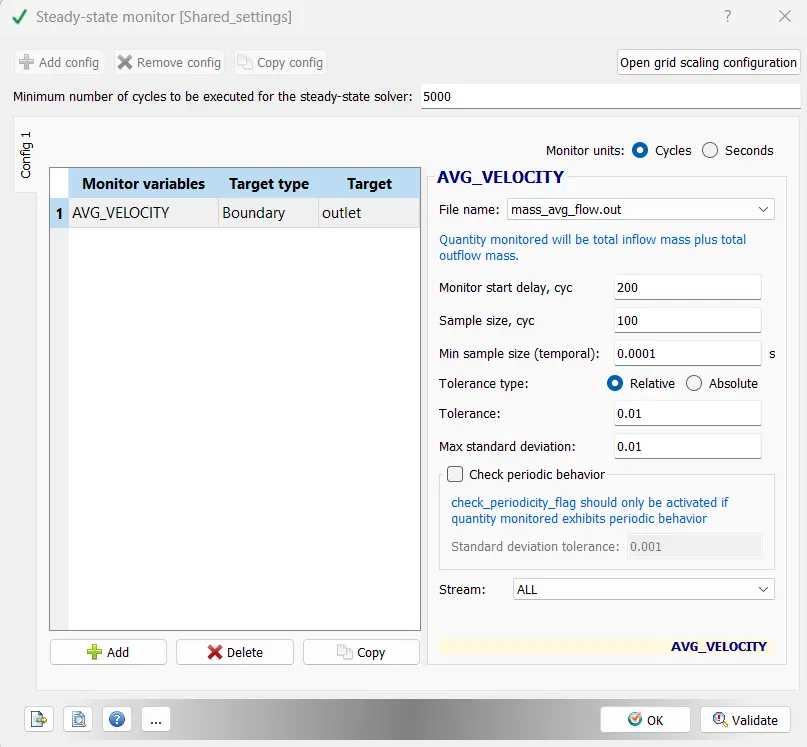
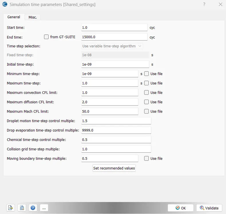
Total number cycle will be 15000, Initial time step 1e-09 which is the smallest time step possible in Converge.
The CFL limit for maximum convection has been set as 1 to control the simulation stability.
Density based solver chosen
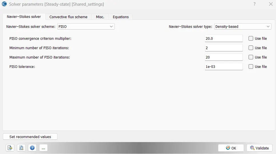
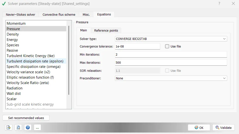
Preconditioner used to be none
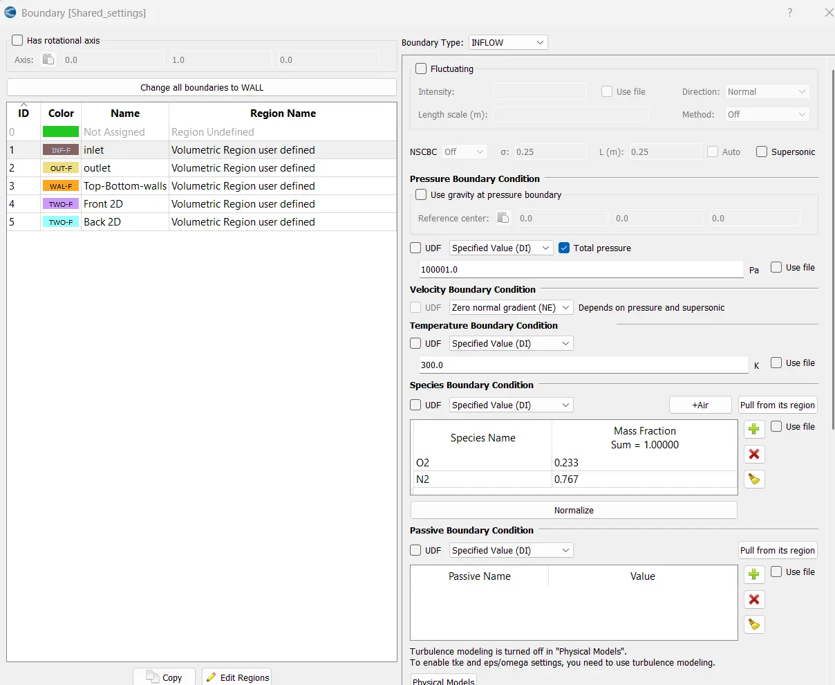
Boundary Conditions
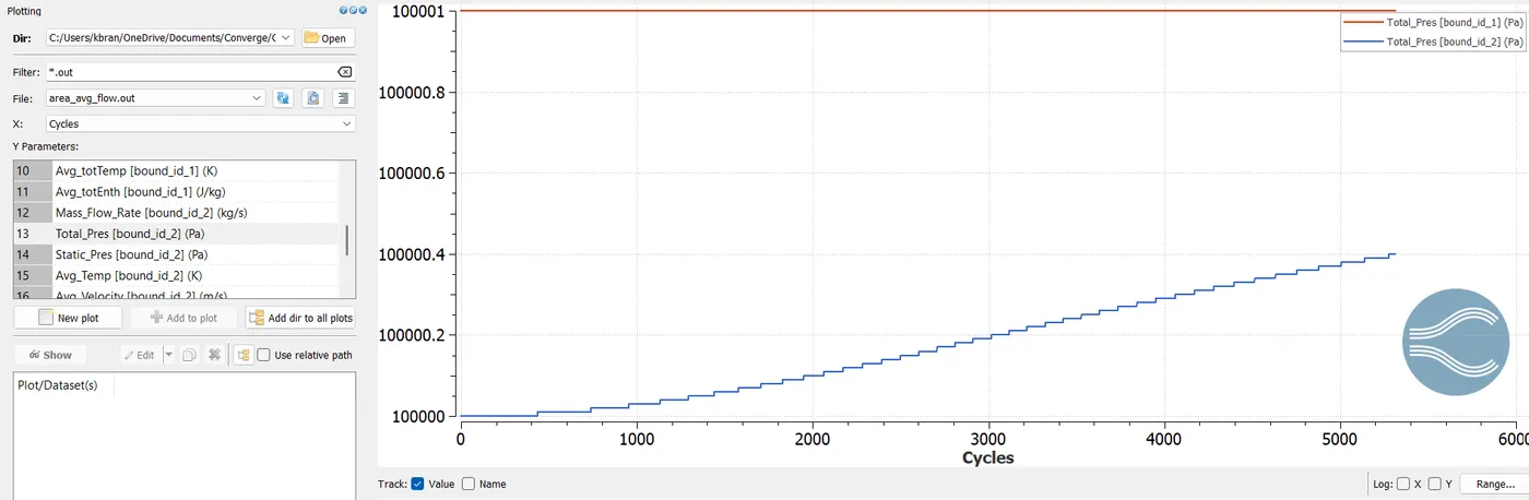
consider 1.00001 bar pressure at inlet. Temperature is 300K and zero normal gradient for velocity boundary condition.
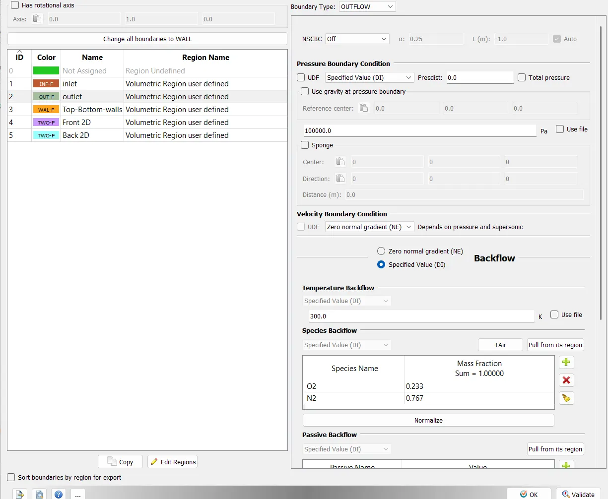
Outlet
Top and bottom wall
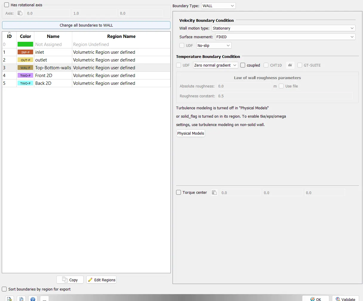
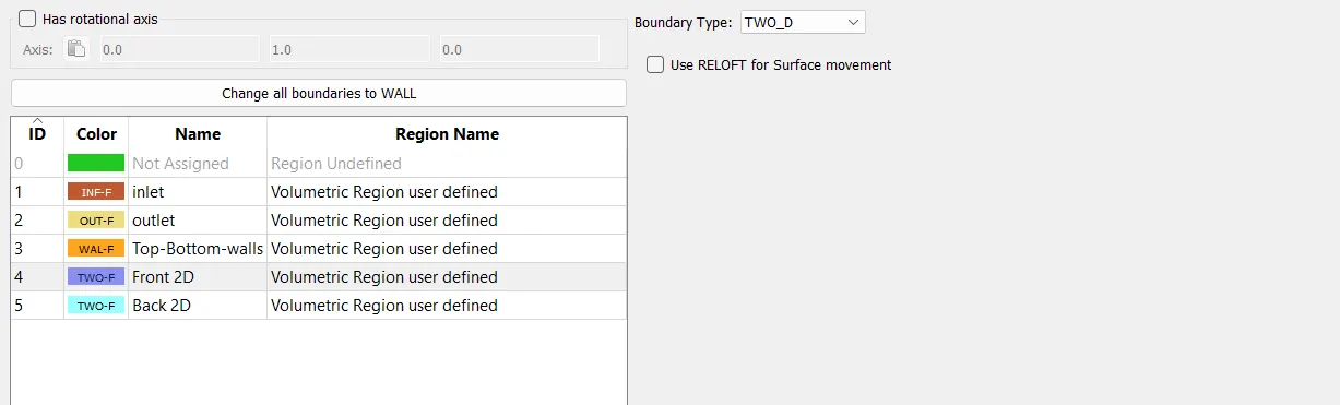
Front and back 2D
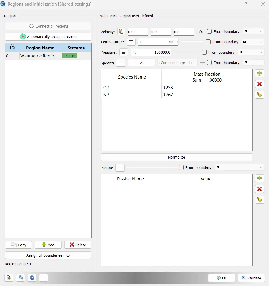
Initial conditions
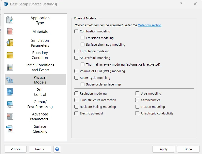
Physical Model
Unchecking the turbulence model.
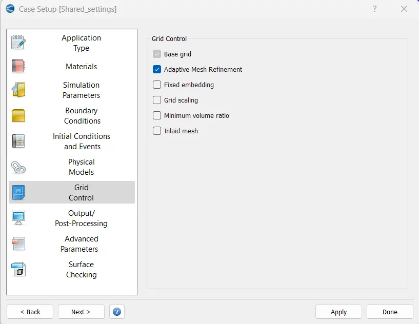
Grid Control
selected adaptive mesh refinement
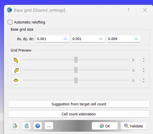
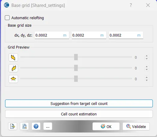
Base Grid
Change the grid size according to mesh size
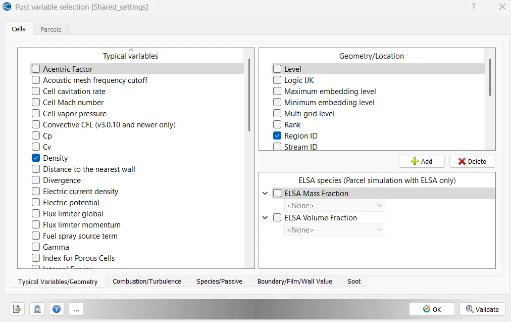
Post processing
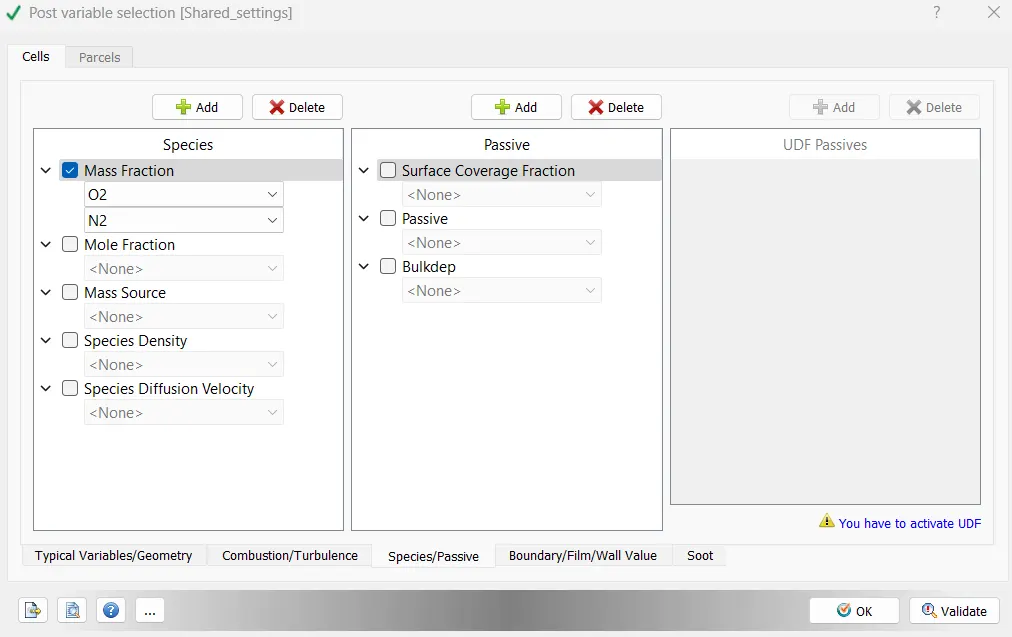
Mass fraction is defined
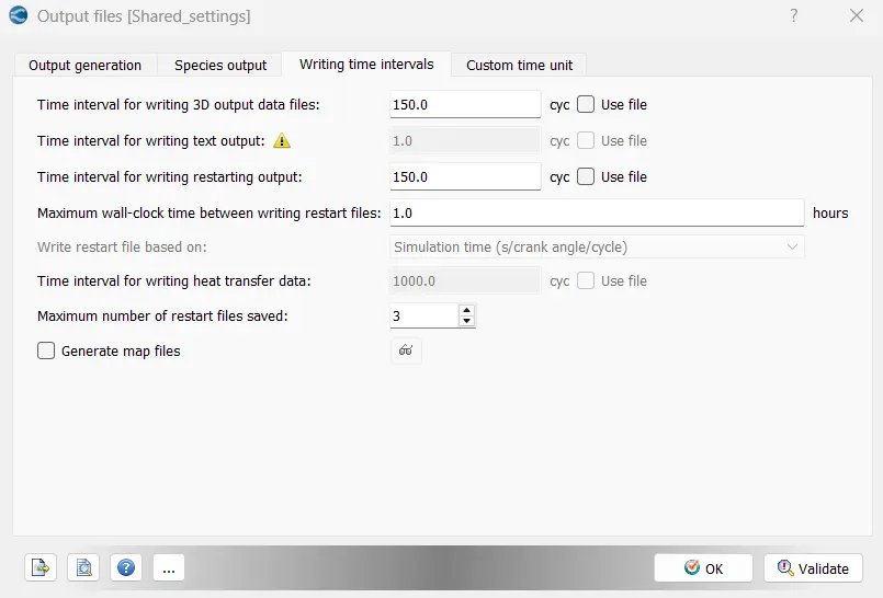
In Output files, the time interval for writing 3D output files & writing restarting output files has been decreased from 1000 to 150 to maintain the 100 output files to post process the simulation results.
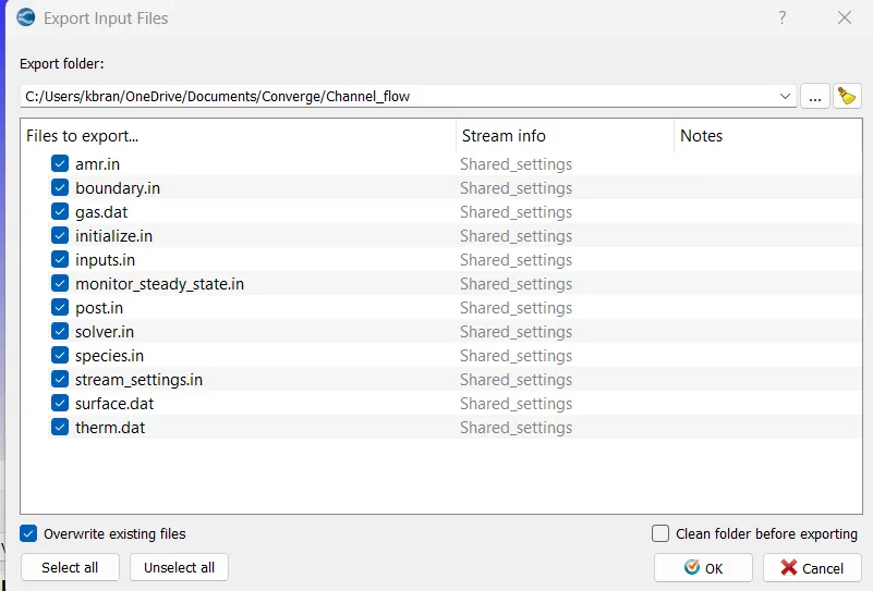
Export the input files
File >export >export input files
These files will be used in the Cygwin to perform the simulation as Converge CFD does not have solver in built.
Simulation,
Go to the Converge installed location
C:\Program Files\Convergent_Science\CONVERGE\3.1.9\bin\intelmpi
Copy the converge.exe files to The input folder.
Open the Cygwin64 terminal, navigate to the Input files folder.
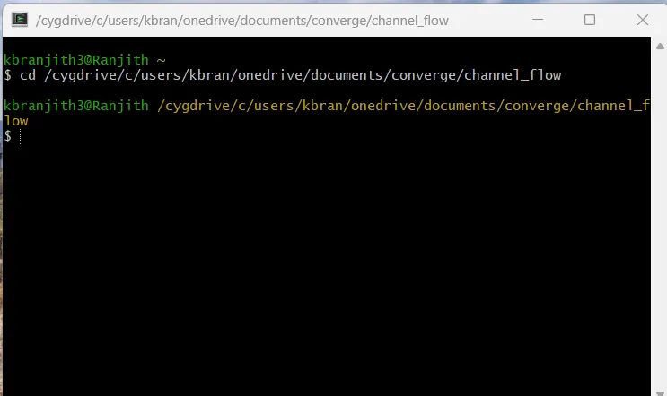
“mpiexec -n 4 converge --license explore” use this command for parallel computing.
Analysis of all the cases
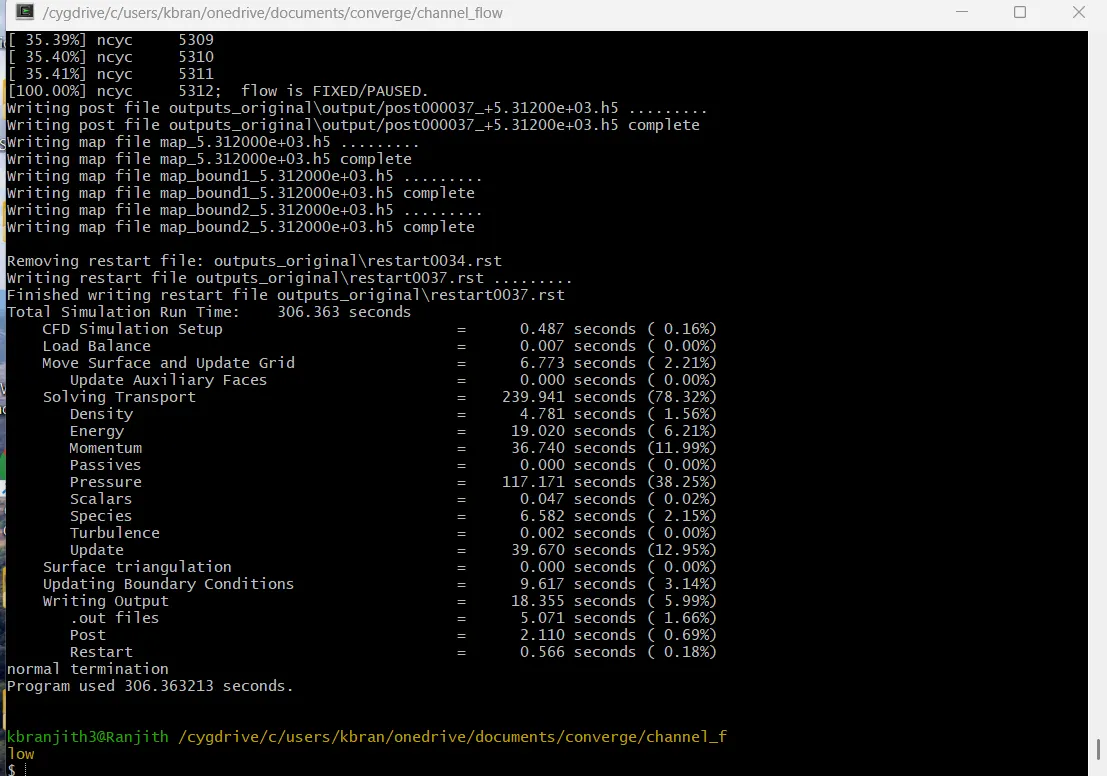
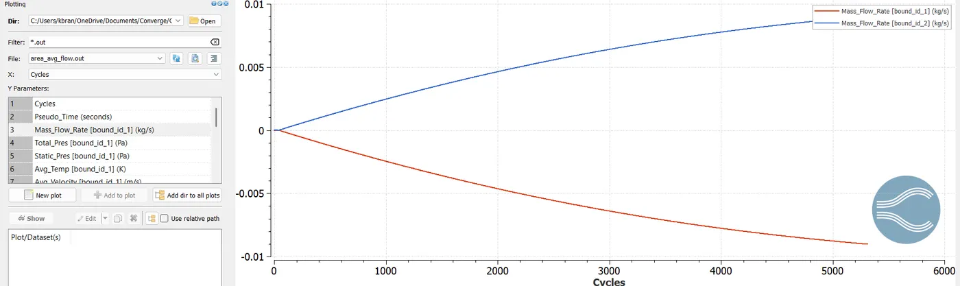
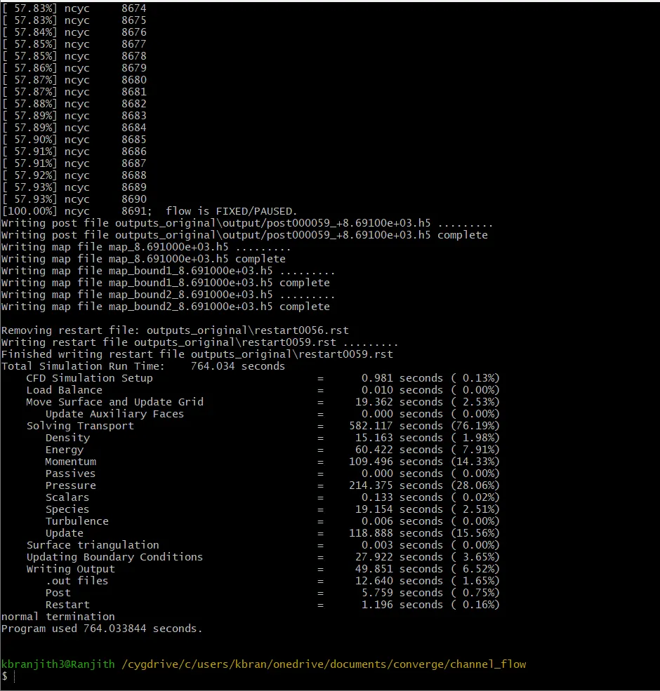
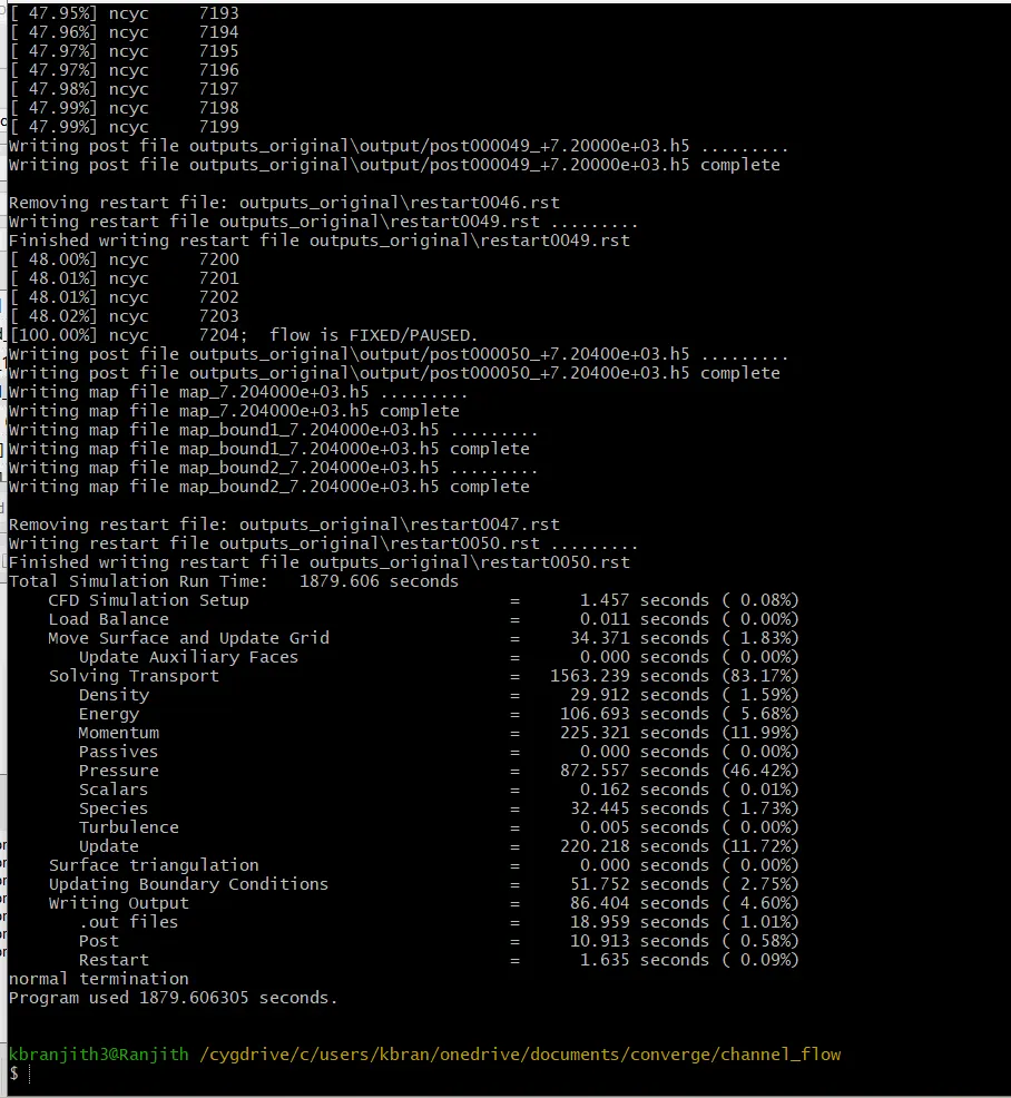
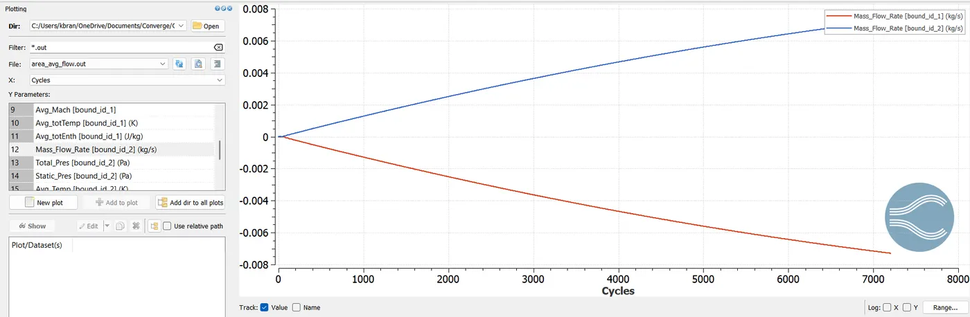
Solution converged at 5312 cycles. Time taken 306.3 seconds
Convert the output files to Paraview VTK file. Navigate the directry to outputfolder.
Select all files. Click on convert.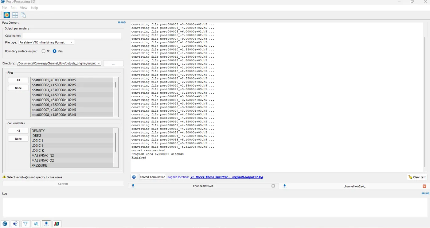
Open Para view, Navigate to output folder. Find the .vtm , group type file. Open it
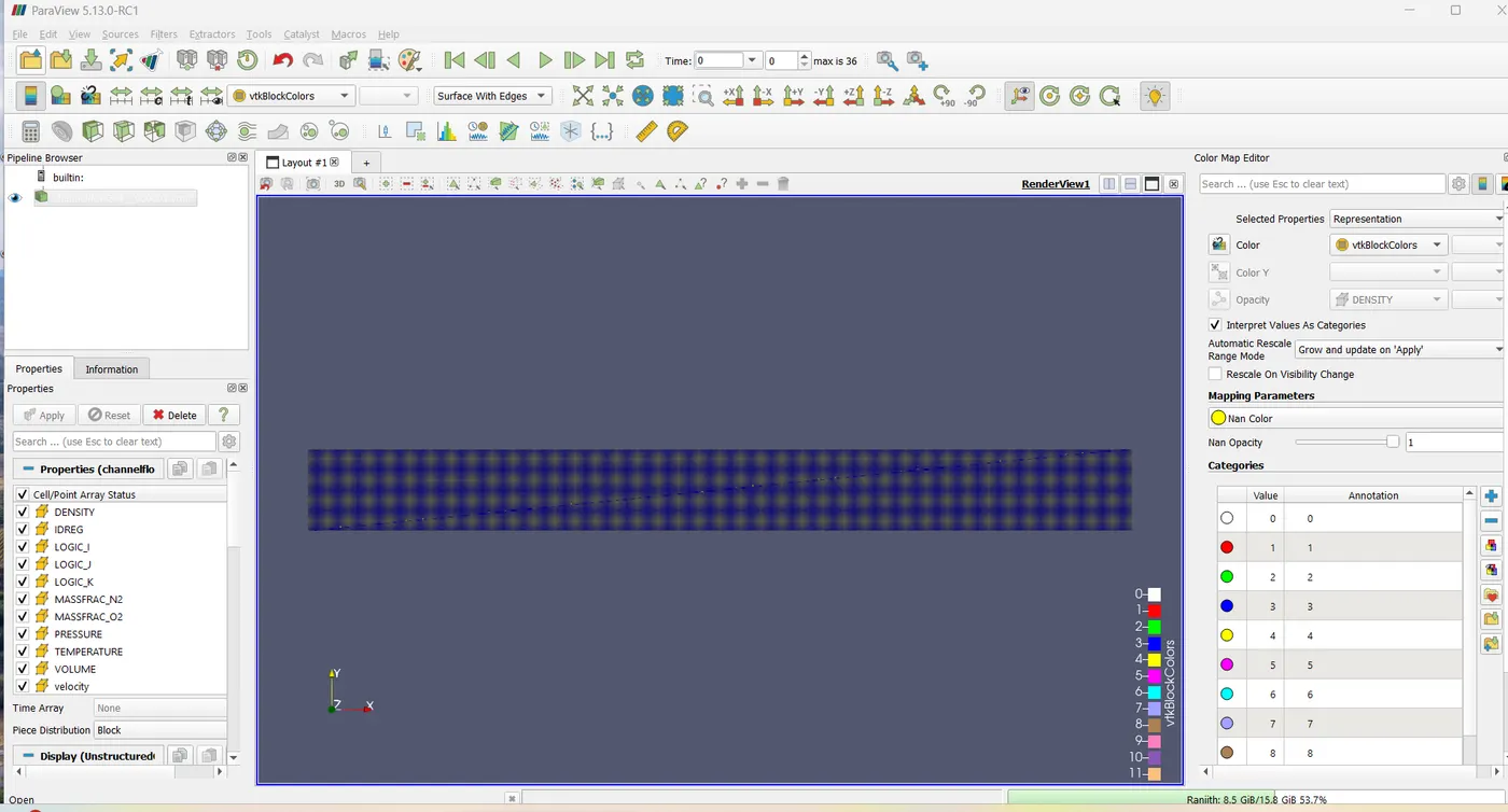
Click on the slice dataset with plane, select the z-normal, uncheck planes, uncheck triangulate the slice. Then apply.
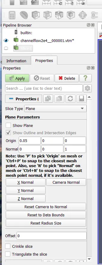
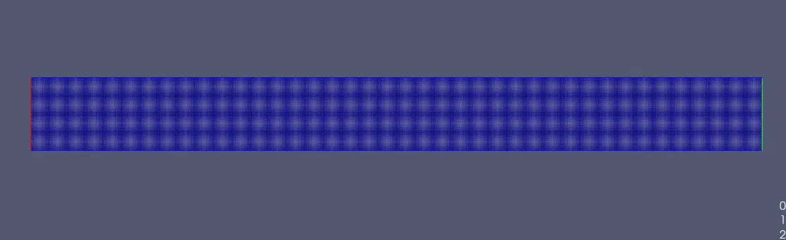
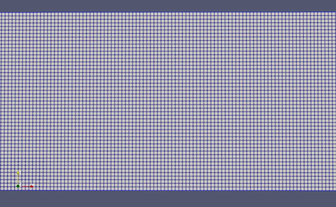
Mesh vie
Results
Case 1
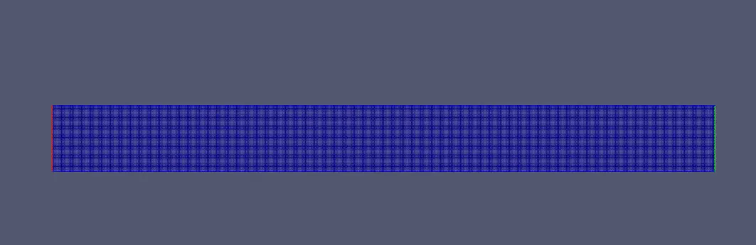
For the Grid size 2e-4m
Mesh view
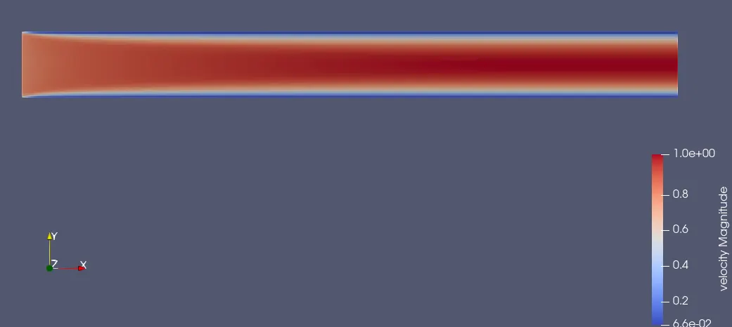
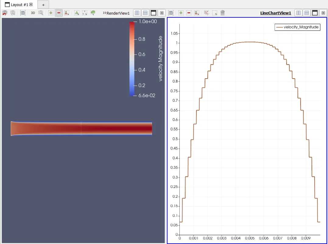
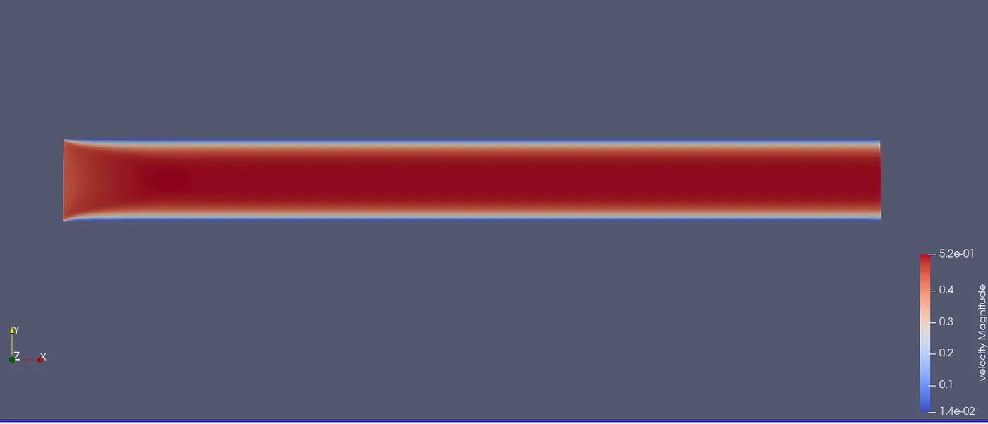
Velocity contour
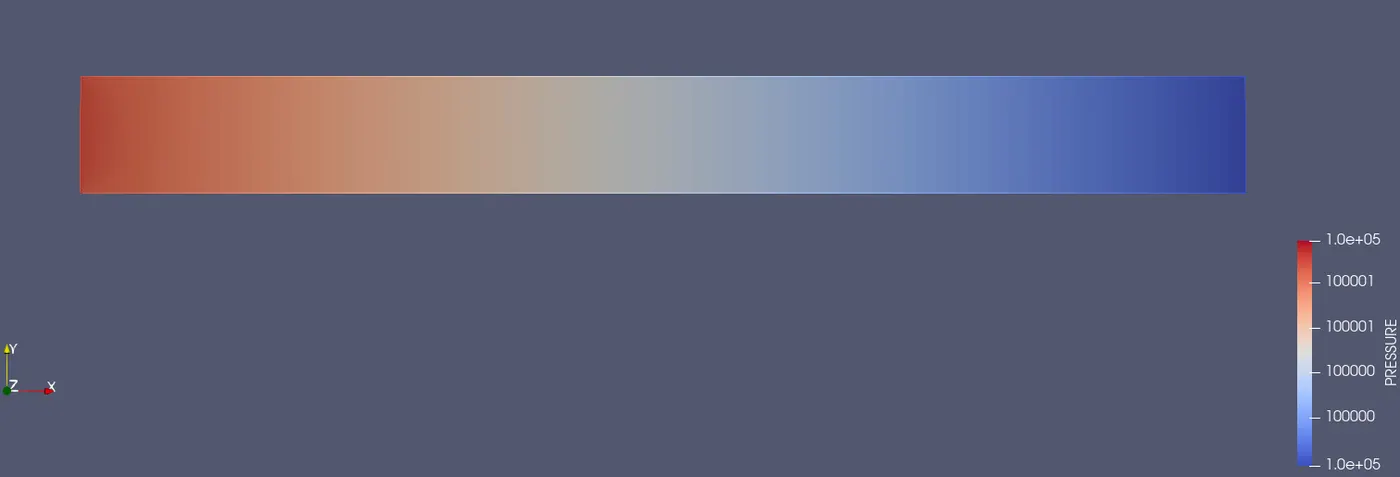
Pressure contour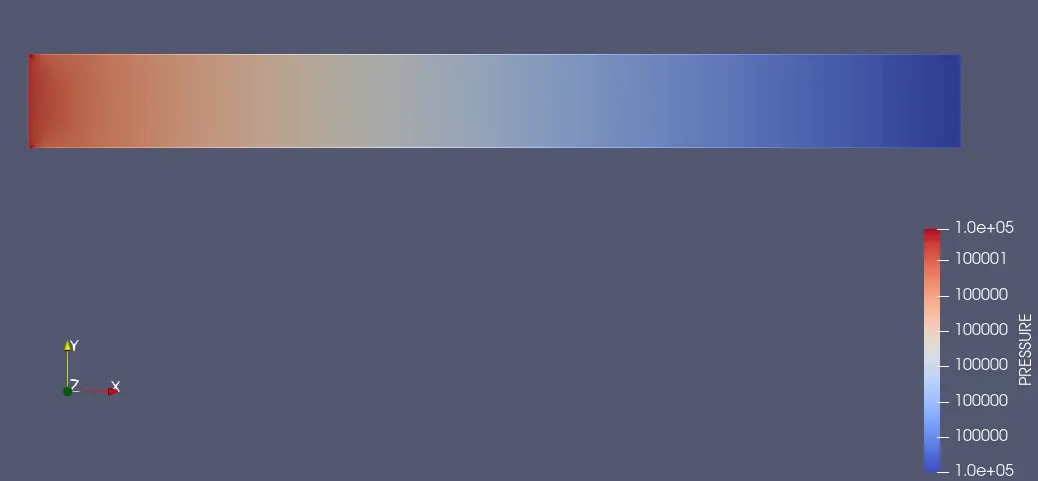
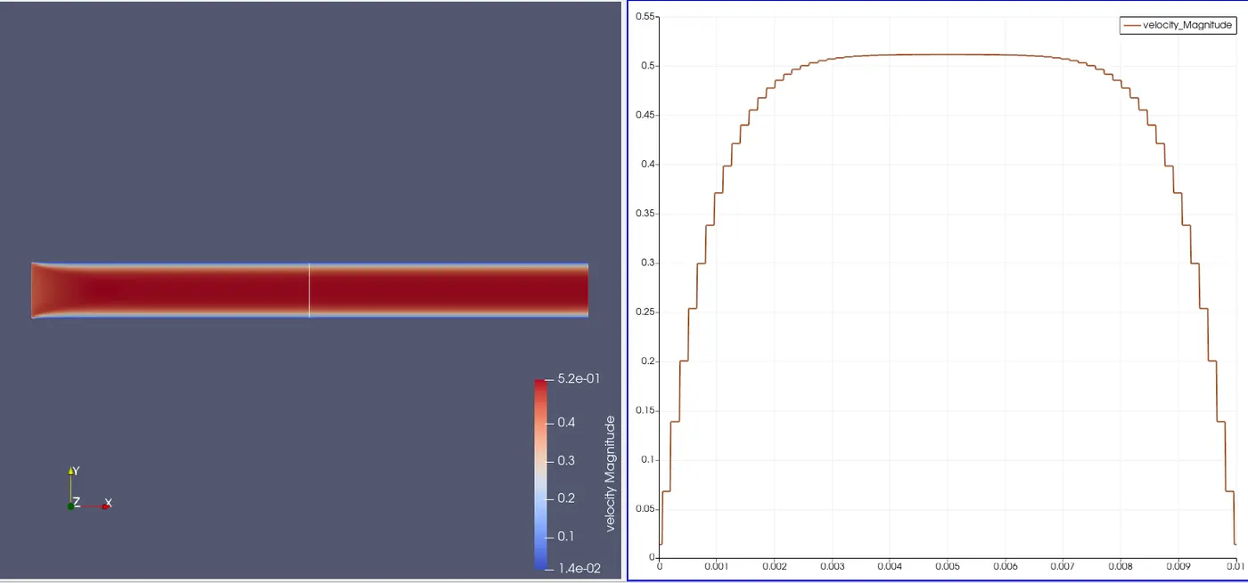
Velocity line plot
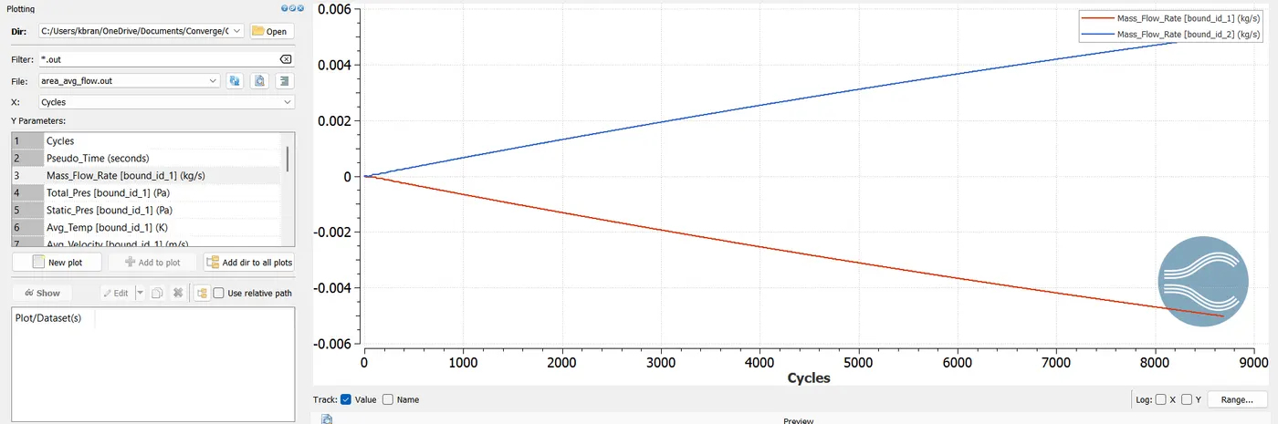
Mass flow rate
Total pressure Plot
Velocity plot
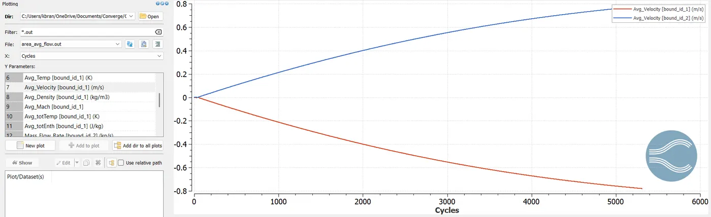
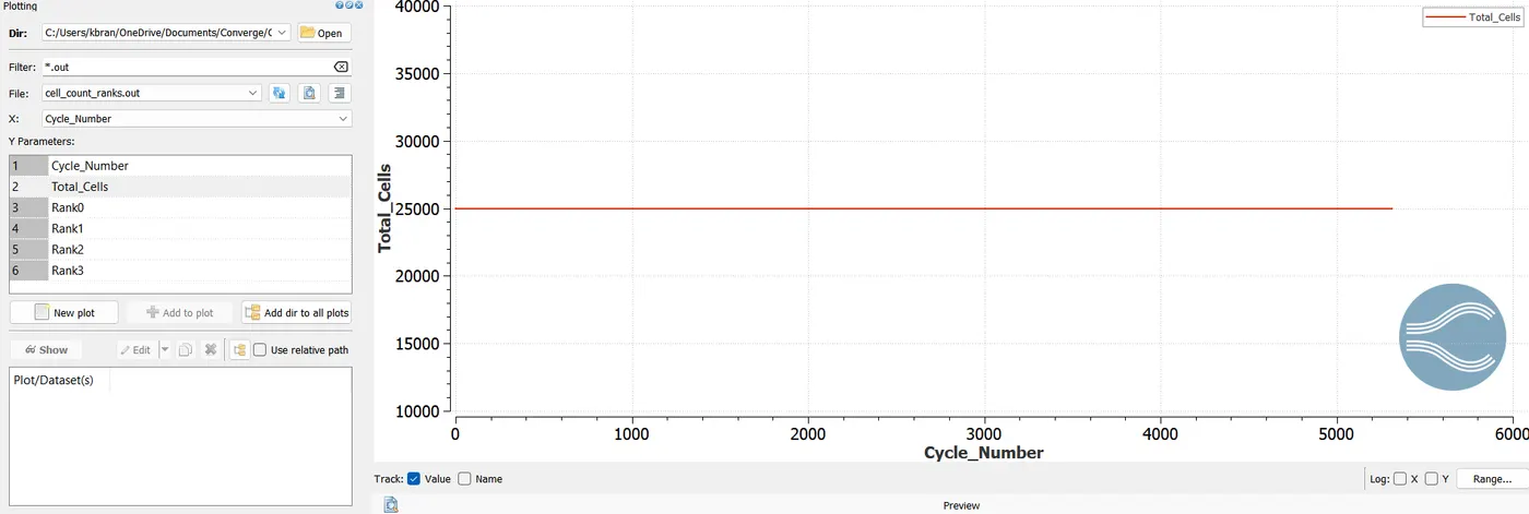
Cell Count
Case 2
For the Grid size 1.5e-4m
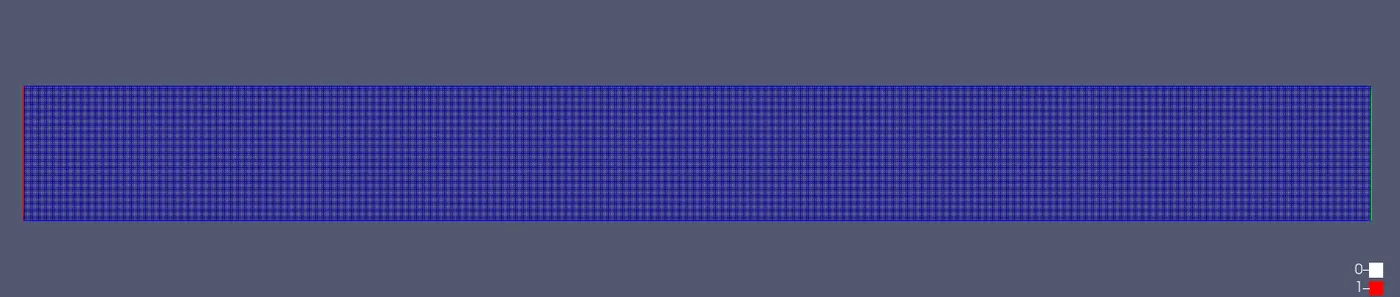
Mesh view
Velocity Contour
Pressure Contour
Velocity plot
Mass flow rate plot
Velocity plot
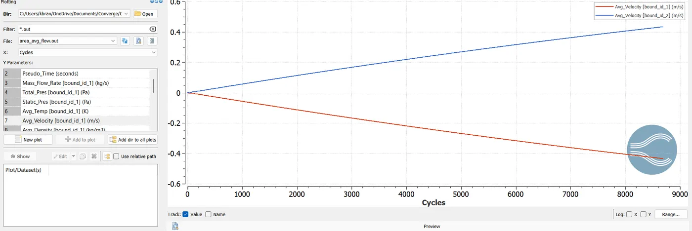
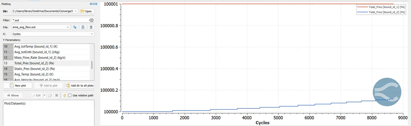
Pressure Plot
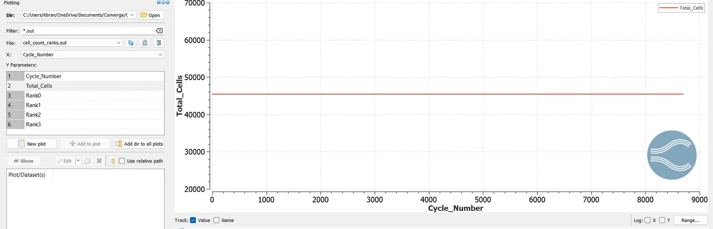
Cell count
Case 3
For the Grid size 1.0e-4m
Mesh View

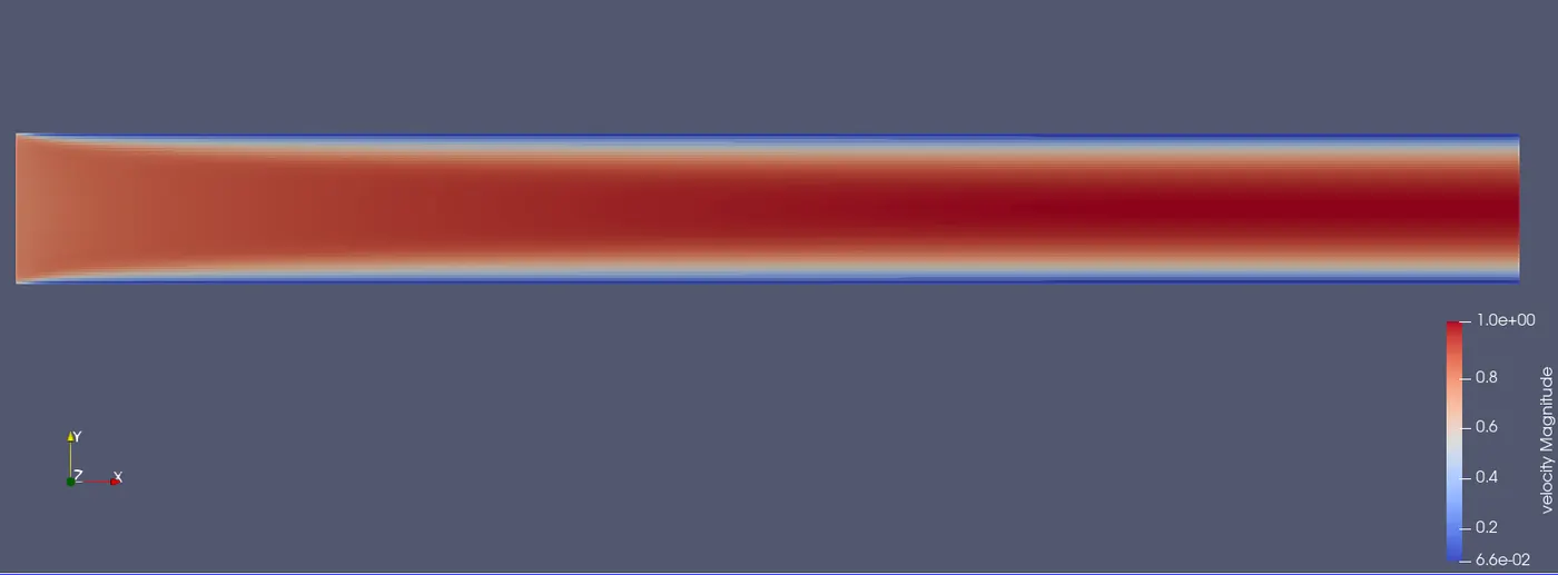
Velocity Contour
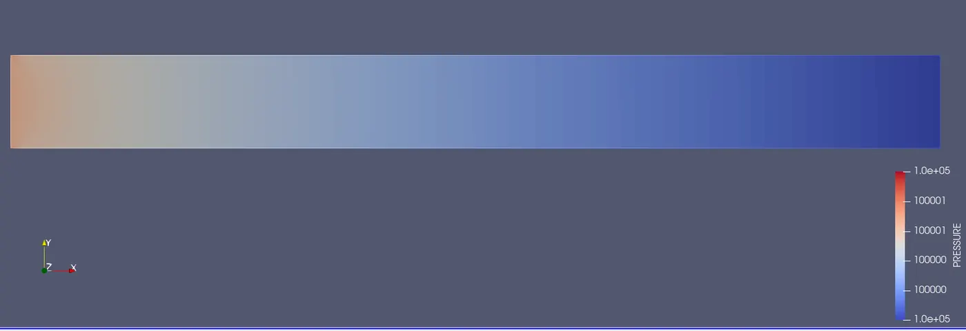
Pressure Contour
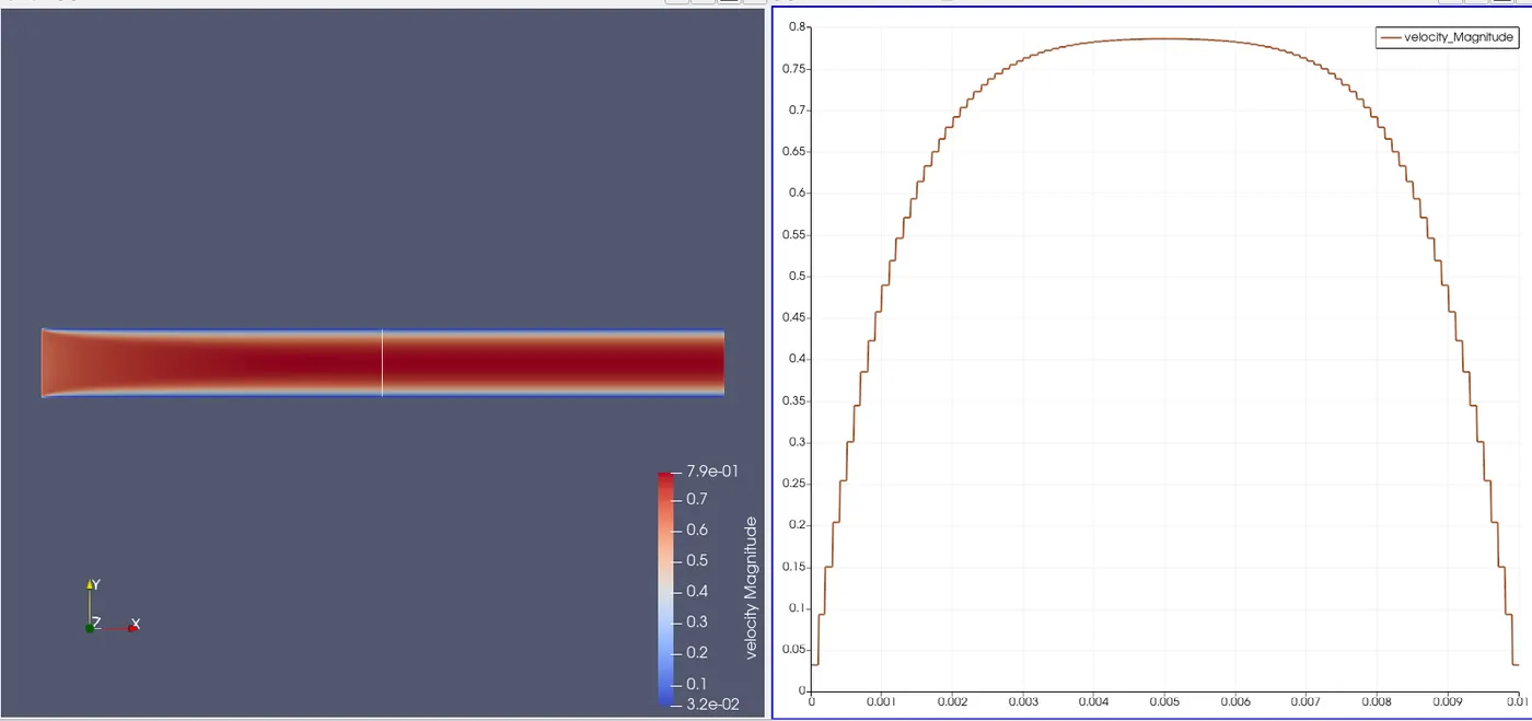
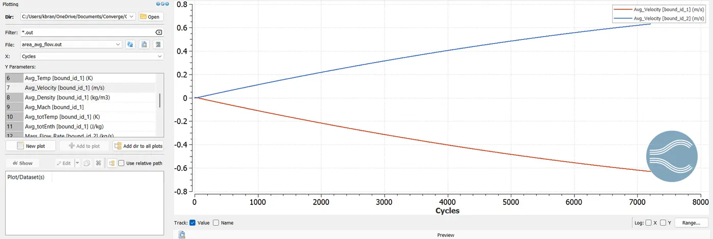
Velocity Plot
Mass Flow rate
Total Pressure plot
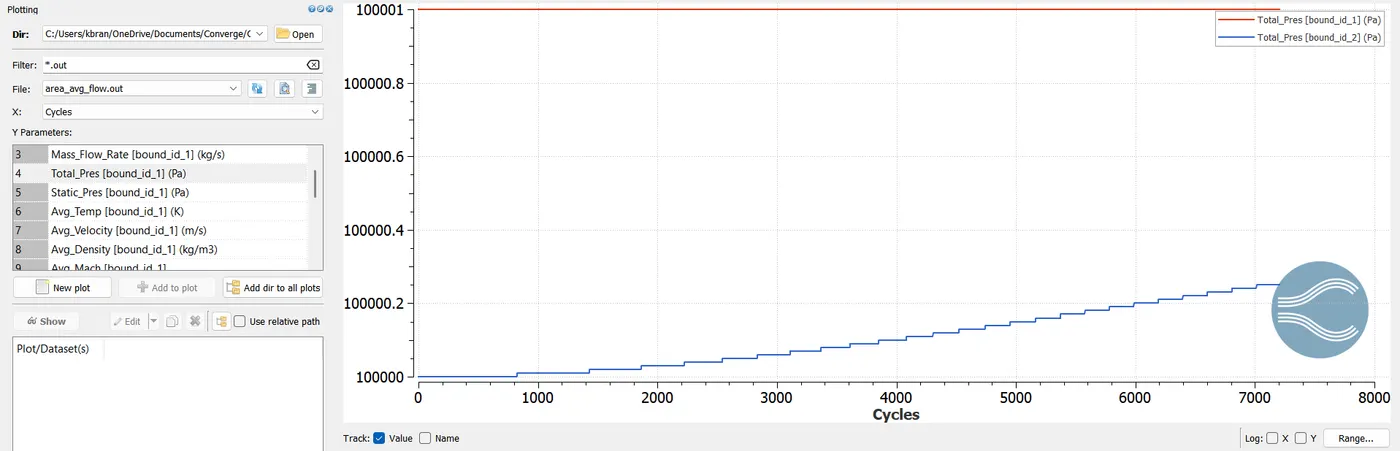
Velocity Plot
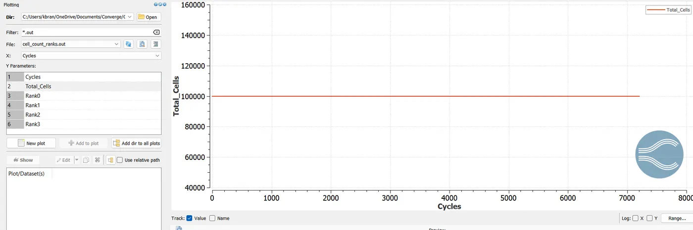
Total cell
All the animation upload in the uploaded in YouTube, link available below
https://youtu.be/XLmKPLXZb9Y (Velocity)
https://youtu.be/w-tASp2JJpU (Pressure)
https://youtu.be/HOObCFrojoY (Density)
Conclusion
From the above analysis, we can conclude that
1. When mesh is refined, simulation run time increases and also accuracy increases
2. By observing Velocity plot (paraview), Velocity magnitude is smoother in case 3 than case 1 Hence, as the grid size increases the results obtained are much clear and accurate.
3. As seen from the velocity animations, the flow at the surface edges has zero velocity as of no slip condition, and as the fluid continues to propagate, its velocity is increased, forming a parabolic velocity profile, which indicates that the maximum velocity is at the center as the streamlines there are least impacted by the wall friction.