Week 5.1 - Mid term project - Solving the steady and unsteady 2D heat conduction problem
Week 5.1 - Mid-term project - Solving the steady and unsteady 2D heat conduction problem
Aim
1. To solve the 2D heat conduction equation by using the point iterative techniques.
2. To implement Jacobi, Gauss-seidel and Successive over-relaxation methods for solving implicit equations.
3. To write code for both implicit and explicit schemes transient analysis.
4. To Compare the convergence rate [Number of iterations] of the steady state and transient [explicit and implicit] simulations and to justify the numeric
Introduction:
The one-dimension heat conduction equation is written as,
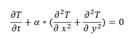
Where T = temperature and α = thermal conductivity.
The heat conduction equation describes how heat (or temperature) is distributed within a given body over time. It’s a partial differential equation that plays a crucial role in understanding thermal behaviour. This law states that the rate of heat transfer through a material is proportional to the negative gradient of temperature and the area through which heat flows.
2D heat conduction equation of steady state
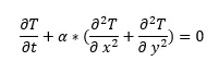
Because of steady state , Properties does not change with time.
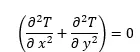
So  ,
,
equation rewrite as,




Where k1 = , k2=
, k2=

As we don't know values at some nodes like T( i+1) and T(j+1) we take guess values.
type of iterative solvers
1. Jacobi Method
In this method, we are using previous iterative values to calculate the present iterative values.
The 2D steady state heat conduction equation for this method,

Gauss-seidel method
In this method, we are using present iterative values to calculate the present iterative values.
The 2D steady state heat conduction equation for this method,

Successive over relaxation method
This method used to solve the equation faster. We can use this method along with Jacobi and Gauss seidel method. We use omega as relaxation coefficient. If omega is less than 1 is called under relaxation. If omega is more than 1, it’s called over relaxation.

Inputs and assumptions
1. the domain length is L = 1m in x and y direction
2. Top Boundary temperature = 600 K; Bottom Boundary temperature = 900 K; Left Boundary temperature = 400 K; Right Boundary temperature = 800 K
3. number of nodes in x and y direction is nx=ny=20
4. error=9e9; tolerance = 1e-4;
Code
The calculation Code for steady state
clear all
close all
clc

tic
% inputs
nx = 20; %total number of nodesin x axis
ny=nx; %total number of nodesin y axis
al=1;  % alpha value; conductivity of material
L=1; %length of plate

%Initializing array
T= 300*ones(nx,ny);

x= linspace(0,L,nx);
y= linspace(0,L,ny);

%calculating the constants
dx=x(2)-x(1);
dy=y(2)-y(1);

k1=(0.5*(dy^2))/((dx^2)+(dy^2));
k2=(0.5*(dx^2))/((dx^2)+(dy^2));

%boundary conditions
Ttop=600;
Tbotm=900;
tleft=400;
Trght=800;

%assigning the boundary condition
T(1,:)=Ttop; %Top boundary Temperature
T(end,:)=Tbotm; %bottom boundary Temperature
T(:,1)=tleft; %left boundary Temperature
T(:,end)=Trght; %Right boundary Temperature

%copying the temperature
Told=T;

iterative_solver = input('enter_the_solver_number: ');
error=9e9;
tol = 1e-4;

%jacobi method

if iterative_solver == 1
    jacobi_iter = 1;
    while (error > tol)
       for i = 2:nx-1
            for j = 2:ny-1
                T(i,j)=(k1*(Told(i-1,j)+Told(i+1,j)))+(k2*(Told(i,j-1)+Told(i,j+1)));
            end
        end

    error = max(max(abs(Told-T)));
    Told=T;
    jacobi_iter = jacobi_iter + 1;
    [c,h]=contourf(x,fliplr(y),T);
    clabel(c,h)
    colormap(jet)
    colorbar;
    xlabel('x-axis')
    ylabel('y-axis')
    computation_time=toc;
    title_text = sprintf('Steady state Jacobi iteration number= %d; computation time: %0.3f s',jacobi_iter,computation_time);
    title(title_text)
    pause(0.00003)
    end
end


%gauss seidel method

if iterative_solver == 2
    gs_iter = 1;
    while (error > tol)
         for i = 2:nx-1
            for j = 2:ny-1
                T(i,j)=(k1*(T(i-1,j)+T(i+1,j)))+(k2*(T(i,j-1)+T(i,j+1)));
            end
        end

    error = max(max(abs(Told-T)));
    Told=T;
    gs_iter = gs_iter + 1;
    [c,h]=contourf(x,fliplr(y),T);
    clabel(c,h)
    colormap(jet)
    colorbar;
    xlabel('x-axis')
    ylabel('y-axis')
    computation_time=toc;
    title_text = sprintf('Steady state Gauss seidel iteration number= %d; computation time: %0.3f s',gs_iter,computation_time);
    title(title_text)
    pause(0.00003)
    end
end


%Successive over relaxation method

omega=1.722; % relaxation coefficient
Tgs=T;
if iterative_solver == 3
    sor_iter = 1;
    while (error > tol)
         for i = 2:nx-1
            for j = 2:ny-1
                Tgs(i,j)=(k1*(T(i-1,j)+T(i+1,j)))+(k2*(T(i,j-1)+T(i,j+1)));
                T(i,j)=(Told(i,j)*(1-omega))+(omega*Tgs(i,j));
            end
        end

    error = max(max(abs(Told-T)));
    Told=T;
    sor_iter = sor_iter + 1;
    [c,h]=contourf(x,fliplr(y),T);
    clabel(c,h)
    colormap(jet)
    colorbar;
    xlabel('x-axis')
    ylabel('y-axis')
    computation_time=toc;
    title_text = sprintf('steady stateGS SOR iteration number= %d; computation time: %0.3f s',sor_iter,computation_time);
    title(title_text)
    pause(0.00003)
    end
end
Results for steady state
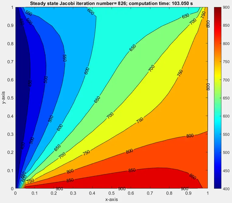
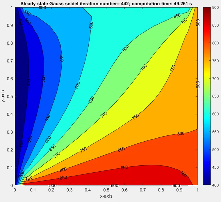
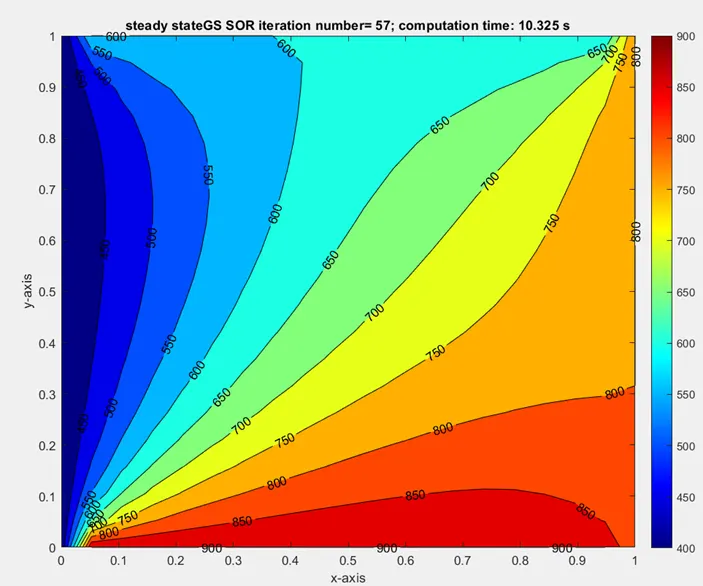
As per the above plots we can observe that number of iteration and computation time is reduced in Gauss Siedel compared to Jacobi method. When we do over relaxation, the number of iteration and computation time further reduced. So, Gauss seidel over relaxation method converged faster than all other method.
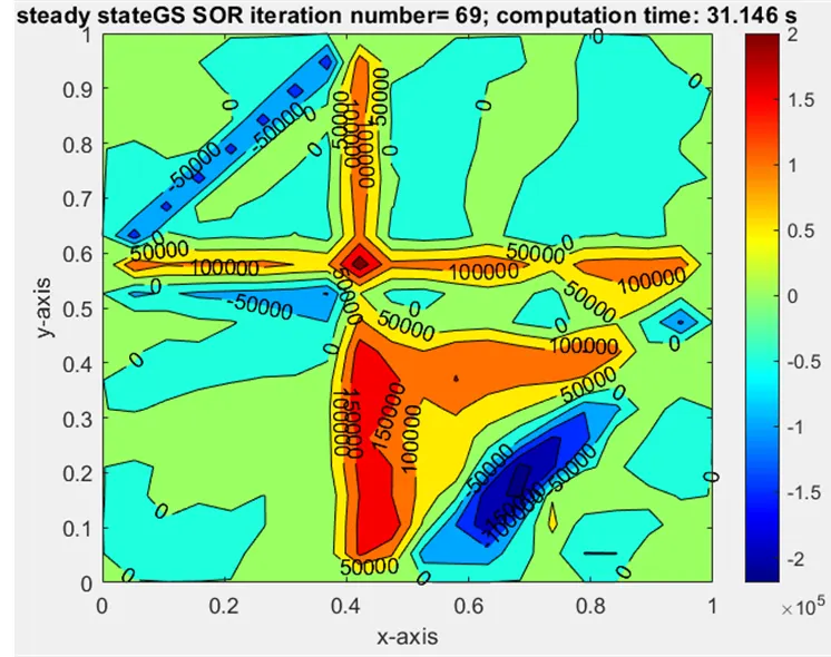
When we do over relaxation to the gauss seidel method, at omega 1.722 we get optimum solution that means number of iteration and computation time reduced and it converged faster. But, if we omega is more than 2 , solution will explode as shown in below picture and it won’t converge.
2D heat conduction equation of transient state
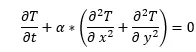
Because of transient state, Properties does change with time.
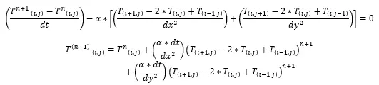
When we apply finite difference central method, equation rewrite as,
Where k1 = , k2=
, k2=


The above equation is implicit transient equation. We need to replace  with
with  in right side of the equation for implicit transient equation.
2D heat conduction equation of transient state explicit form

Inputs and assumptions
1. the domain length is L = 1m in x and y direction
2. Top Boundary temperature = 600 K; Bottom Boundary temperature = 900 K; Left Boundary temperature = 400 K; Right Boundary temperature = 800 K
3. number of nodes in x and y direction is nx=ny=20
4. error=9e9; tolerance = 1e-4;
5. Simulation run time, t = 0.14 seconds.
6. time steps dt= 1e-4;
Code
The calculation Code for transient state explicit form
clear all
close all
clc

tic
% inputs
nx = 20; %total number of nodesin x axis
ny=nx; %total number of nodesin y axis
t=0.14; % simulation run time
dt=1e-4; %time step
al=1;  % alpha value; conductivity of material
L=1; %length of plate

%Initializing array
T= 300*ones(nx,ny);

x= linspace(0,L,nx);
y= linspace(0,L,ny);

%calculating the constants
dx=x(2)-x(1);
dy=y(2)-y(1);

%boundary conditions
Ttop=600;
Tbotm=900;
tleft=400;
Trght=800;

%assigning the boundary condition
T(1,:)=Ttop; %Top boundary Temperature
T(end,:)=Tbotm; %bottom boundary Temperature
T(:,1)=tleft; %left boundary Temperature
T(:,end)=Trght; %Right boundary Temperature

%copying the temperature
T_prev_dt=T;

%Time step and consstant calculation

nt=t/dt;
k1=(al*dt)/(dx^2);
k2=(al*dt)/(dy^2);


%explicit method

for k = 1:nt

           for i = 2:nx-1
                for j = 2:ny-1
                    term1=(1+(2*k1)+(2*k2))^-1;
                    term2=k1*term1;
                    term3=k2*term1;
                    H=(T_prev_dt(i-1,j)+T_prev_dt(i+1,j));
                    V=(T_prev_dt(i,j-1)+T_prev_dt(i,j+1));
                    T(i,j)=(T_prev_dt(i,j)*term1)+(H*term2)+(V*term3);
                end
           end

        T_prev_dt=T;
        [c,h]=contourf(x,fliplr(y),T);
        clabel(c,h)
        colormap(jet)
        colorbar;
        xlabel('x-axis')
        ylabel('y-axis')
        computation_time=toc;
        title_text = sprintf('explicit transient state computation time: %0.3f s',computation_time);
        title(title_text)
        pause(0.00003)
end
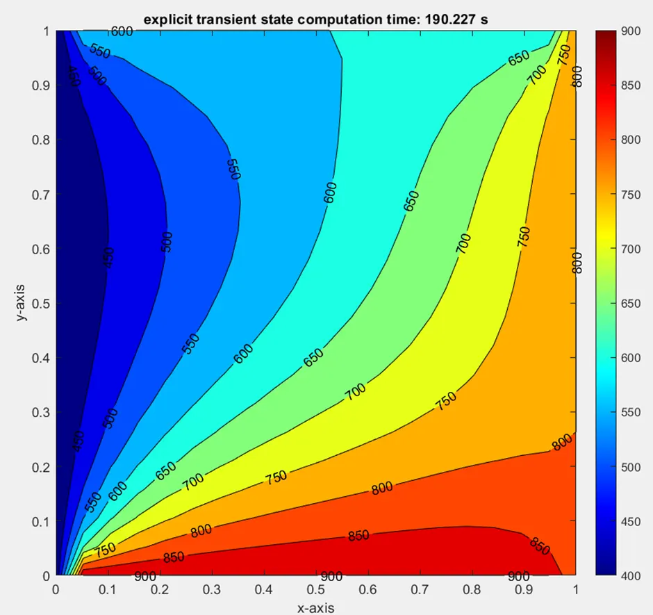
Results for transient state explicit
2D heat conduction equation of transient state implicit form

Code
The calculation Code for transient state implicit form
clear all
close all
clc
tic
% inputs
nx = 20; %total number of nodesin x axis
ny=nx; %total number of nodesin y axis
t=0.14; % simulation run time
dt=1e-4; %time step
al=1; % alpha value; conductivity of material
L=1; %length of plate
%Initializing array
T= 300*ones(nx,ny);
x= linspace(0,L,nx);
y= linspace(0,L,ny);
%calculating the constants
dx=x(2)-x(1);
dy=y(2)-y(1);
%boundary conditions
Ttop=600;
Tbotm=900;
tleft=400;
Trght=800;
%assigning the boundary condition
T(1,:)=Ttop; %Top boundary Temperature
T(end,:)=Tbotm; %bottom boundary Temperature
T(:,1)=tleft; %left boundary Temperature
T(:,end)=Trght; %Right boundary Temperature
%copying the temperature
Told=T;
T_prev_dt=T;
iterative_solver = input('enter_the_solver_number: ');
error=9e9;
tol = 1e-4;
%Time step and consstant calculation
nt=t/dt;
k1=(al*dt)/(dx^2);
k2=(al*dt)/(dy^2);
%jacobi method
if iterative_solver == 1
jacobi_iter = 1;
for k = 1:nt
error=9e9;
while (error > tol)
for i = 2:nx-1
for j = 2:ny-1
term1=(1+(2*k1)+(2*k2))^-1;
term2=k1*term1;
term3=k2*term1;
H=(Told(i-1,j)+Told(i+1,j));
V=(Told(i,j-1)+Told(i,j+1));
T(i,j)=(T_prev_dt(i,j)*term1)+(H*term2)+(V*term3);
end
end
error = max(max(max(abs(Told-T))));
Told=T;
jacobi_iter = jacobi_iter + 1;
[c,h]=contourf(x,fliplr(y),T);
clabel(c,h)
colormap(jet)
colorbar;
xlabel('x-axis')
ylabel('y-axis')
computation_time=toc;
title_text = sprintf('Jacobi iteration number= %d; computation time: %0.3f s',jacobi_iter,computation_time);
title(title_text)
pause(0.00003)
end
T_prev_dt=T;
end
end
%gauss seidel method
if iterative_solver == 2
gs_iter = 1;
for k=1:nt
error=9e9;
while (error > tol)
for i = 2:nx-1
for j = 2:nx-1
term1=(1+(2*k1)+(2*k2))^-1;
term2=k1*term1;
term3=k2*term1;
H=(T(i-1,j)+T(i+1,j));
V=(T(i,j-1)+T(i,j+1));
T(i,j)=(T_prev_dt(i,j)*term1)+(H*term2)+(V*term3);
end
end
error = max(max(abs(Told-T)));
Told=T;
gs_iter = gs_iter + 1;
[c,h]=contourf(x,fliplr(y),T);
clabel(c,h)
colormap(jet)
colorbar;
xlabel('x-axis')
ylabel('y-axis')
computation_time=toc;
title_text = sprintf('Gauss seidel iteration number= %d; computation time: %0.3f s',gs_iter,computation_time);
title(title_text)
pause(0.00003)
end
T_prev_dt=T;
end
end
%Successive over relaxation method
omega=1.055; % relaxation coefficient
Tgs=T;
if iterative_solver == 3
sor_iter = 1;
for k=1:nt
error=9e9;
while (error > tol)
for i = 2:nx-1
for j = 2:ny-1
term1=(1+(2*k1)+(2*k2))^-1;
term2=k1*term1;
term3=k2*term1;
H=(T(i-1,j)+T(i+1,j));
V=(T(i,j-1)+T(i,j+1));
Tgs(i,j)=(T_prev_dt(i,j)*term1)+(H*term2)+(V*term3);
T(i,j)=(Told(i,j)*(1-omega))+(omega*Tgs(i,j));
end
end
error = max(max(abs(Told-T)));
Told=T;
sor_iter = sor_iter + 1;
[c,h]=contourf(x,fliplr(y),T);
clabel(c,h)
colormap(jet)
colorbar;
xlabel('x-axis')
ylabel('y-axis')
computation_time=toc;
title_text = sprintf('GS SOR iteration number= %d; computation time: %0.3f s',sor_iter,computation_time);
title(title_text)
pause(0.00003)
end
T_prev_dt=T;
end
endResults for transient state implicit form
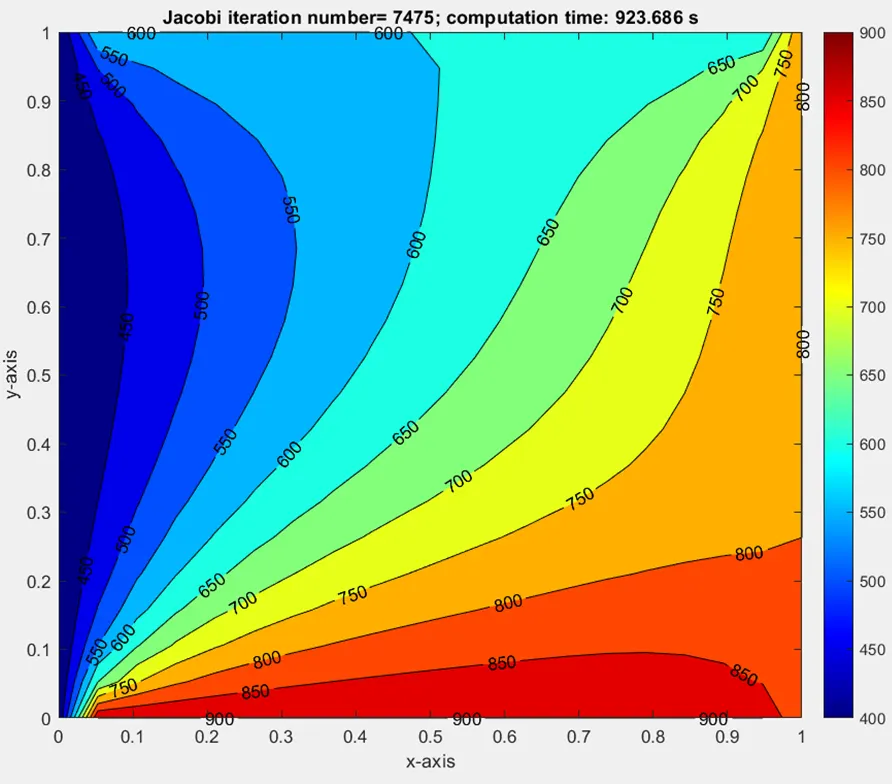
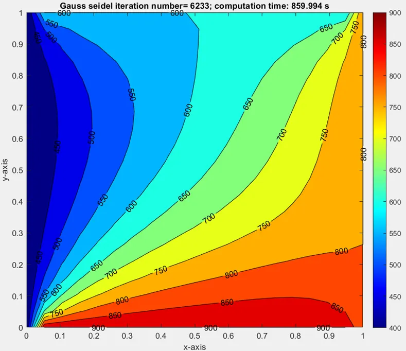
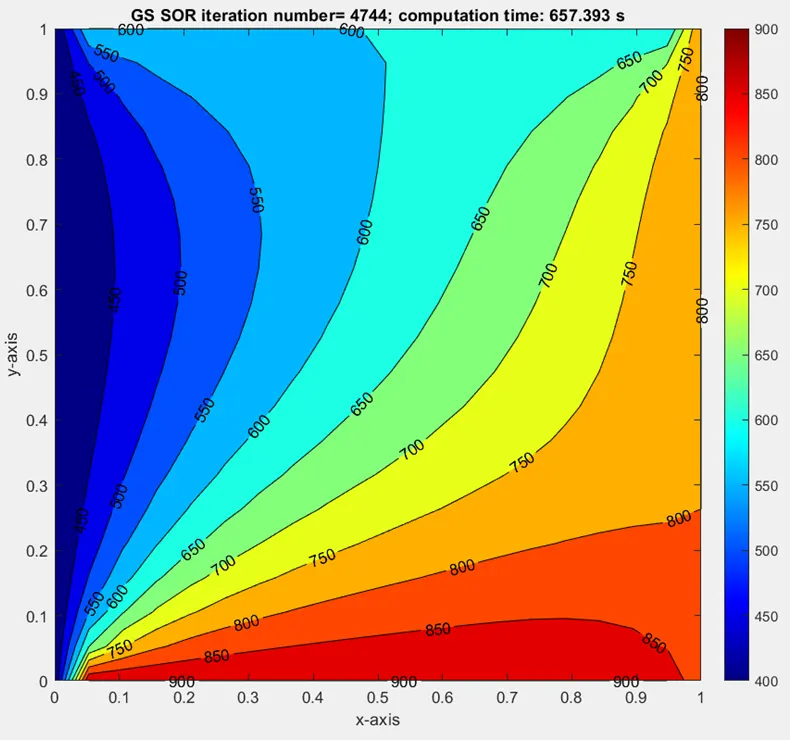
By observing the above plots, number of iteration and computed time is Gauss seidel over relaxation method reduced than other methods. At relaxation coefficient 1.055 we get optimum number of iteration and computation time. At Relaxation coefficient 1.9, solution will blow up.