Aim:

1. To Run the simulation by varying the velocity from 1m/sec to 5m/sec for at least 3 velocities and discuss the results.

2. To Find out the maximum temperature and heat transfer coefficient attained by the processor.

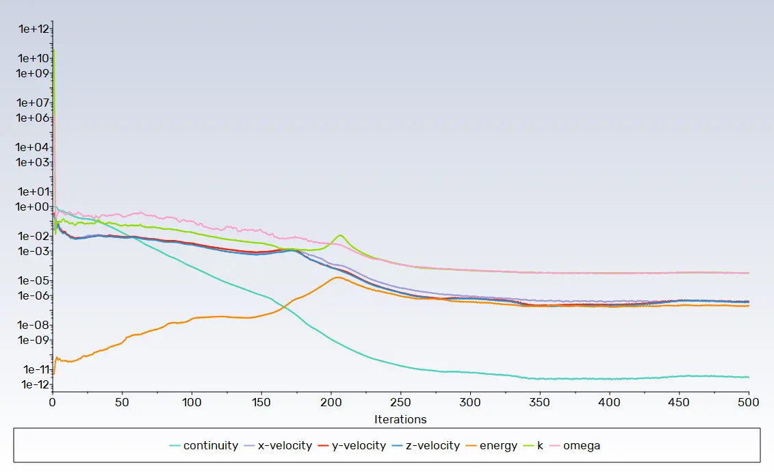
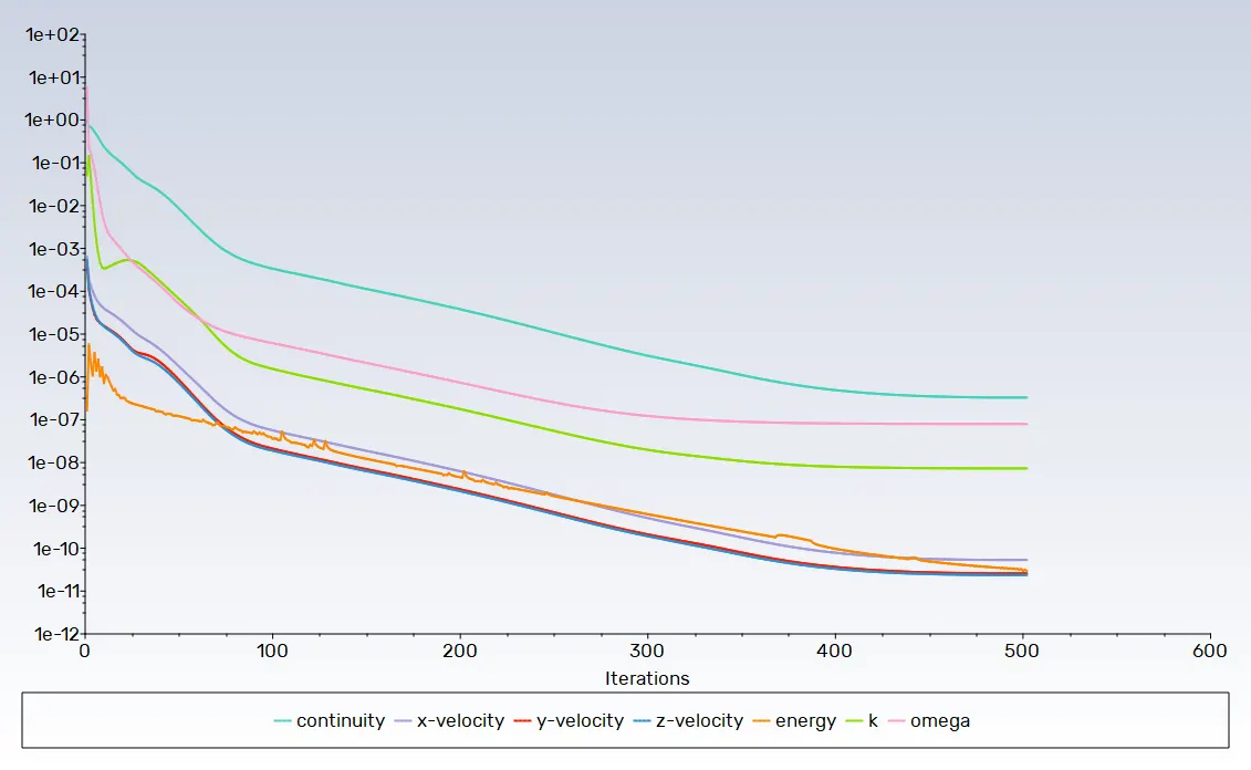
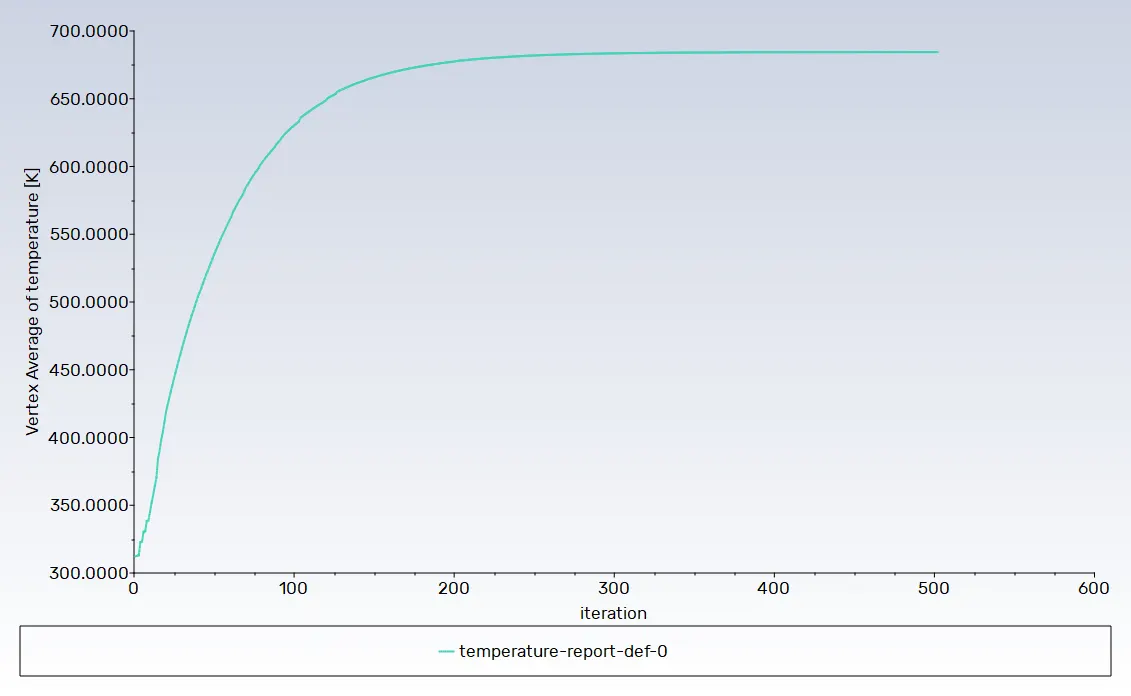
3. To Prove that the simulation has achieved convergence with appropriate images and plots.

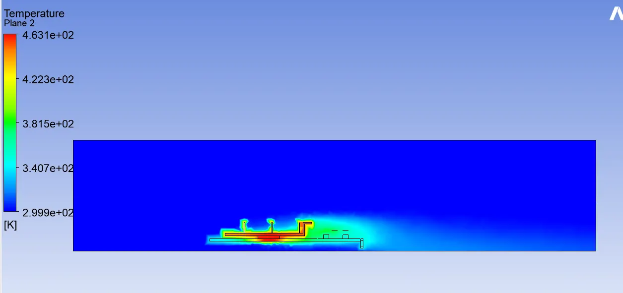
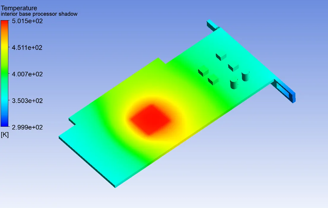
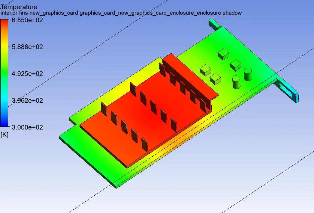
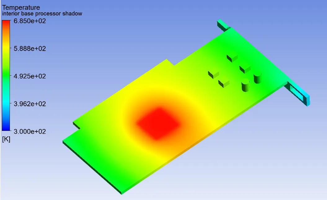
4. To Identify potential hotspots on the model.

Introduction:

Heat Transfer in a Fluid

Due to the fluid motion, three contributions to the heat equation are included:

· The transport of fluid implies energy transport too, which appears in the heat equation as the convective contribution. Depending on the thermal properties on the fluid and on the flow regime, either the convective or the conductive heat transfer can dominate.

· The viscous effects of the fluid flow produce fluid heating. This term is often neglected, nevertheless, its contribution is noticeable for fast flow in viscous fluids.

· As soon as a fluid density is temperature-dependent, a pressure work term contributes to the heat equation. This accounts for the well-known effect that, for example, compressing air produces heat.

Conjugate-Heat-Transfer

Conjugate heat transfer (CHT) refers to the simultaneous transfer of heat between a solid and a fluid. This process is crucial in many engineering applications, such as heat exchangers, electronic cooling systems, and combustion engines.

In solids, heat transfer typically occurs through conduction, while in fluids, it happens through convection. Conjugate heat transfer combines these two mechanisms to provide a comprehensive understanding of the thermal interactions between solids and fluids.

Geometry

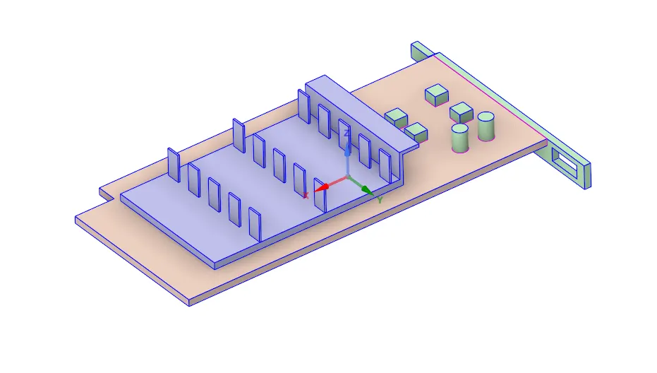
The geometry considered for the current study is a simplified model of the graphics card. The entire card can be classified into three major regions: 1) base of the card, 2) processor and 3) fins

Materials

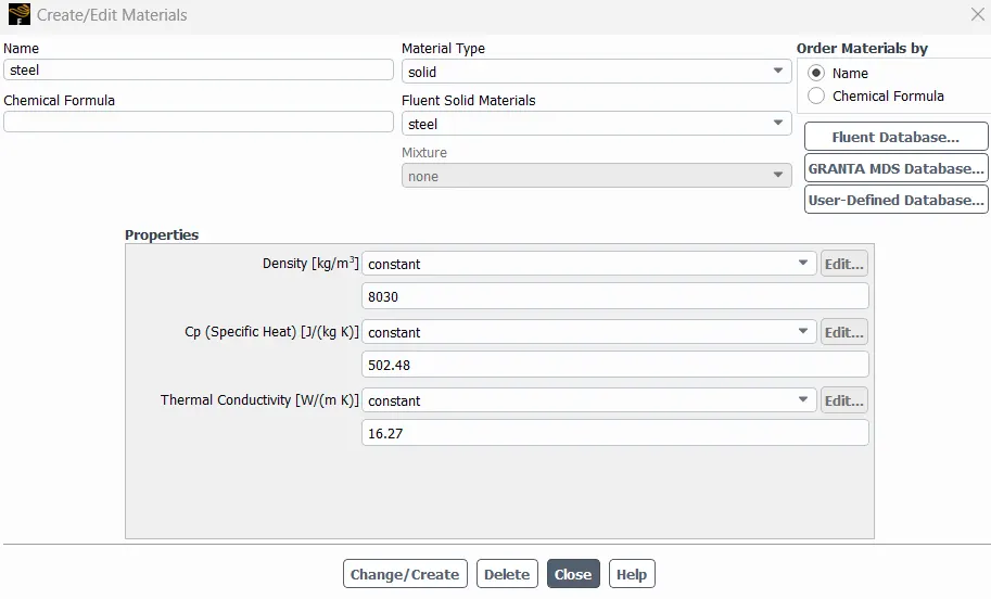
Base: Steel

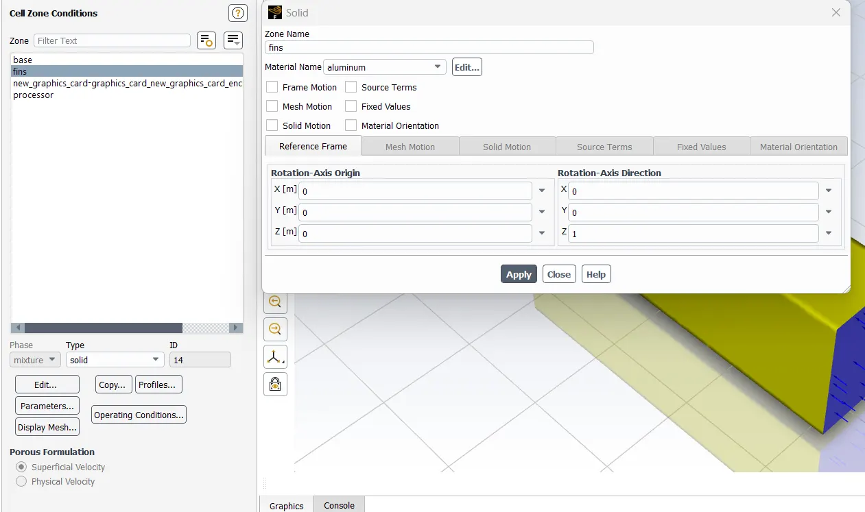
Fins: Aluminum

Processor: Silicon-Pure

Processer considered as energy source. It produces the heat due to electrical power supply which is assumed to be 20kW. Fins are above the processor which helps the convection cooling.

Electrical energy in processor assumed it will completely converted to thermal energy. From simple energy density equation

The working fluid which flows in the enclosure for cooling the card is standard air from the Fluent database

Geometry/Model

Graphics Card Assembly

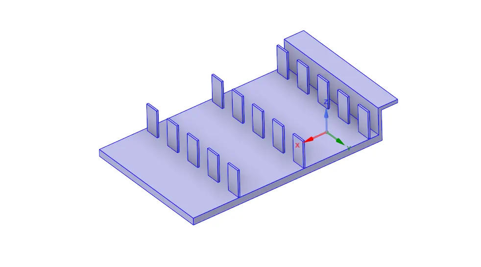
Fins

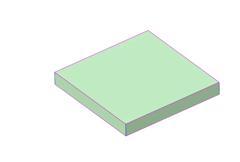
Processor

Base

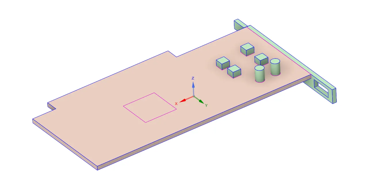
Step Involved in modifying the geometry in space claim

Import the model into space claim. select the share option on workbench for the mesh to be conformal

Physics /Mesh Setup

Mesh

Case1

We are using the default mesh setting. Mesh size is 2.5mm.

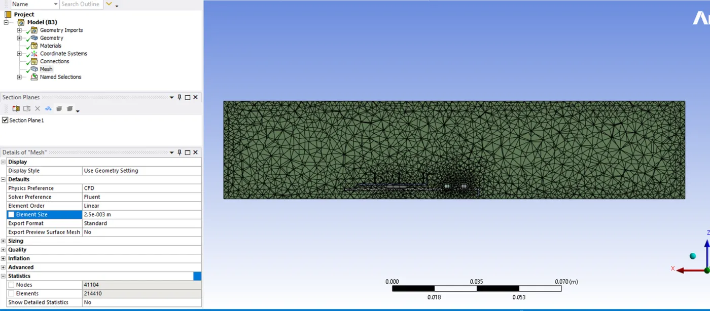
Closer view on Graphics card Assembly

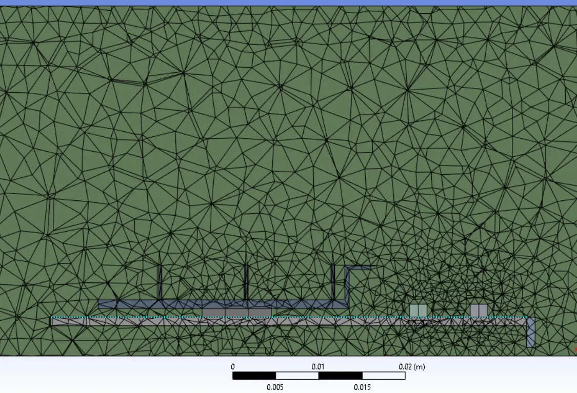
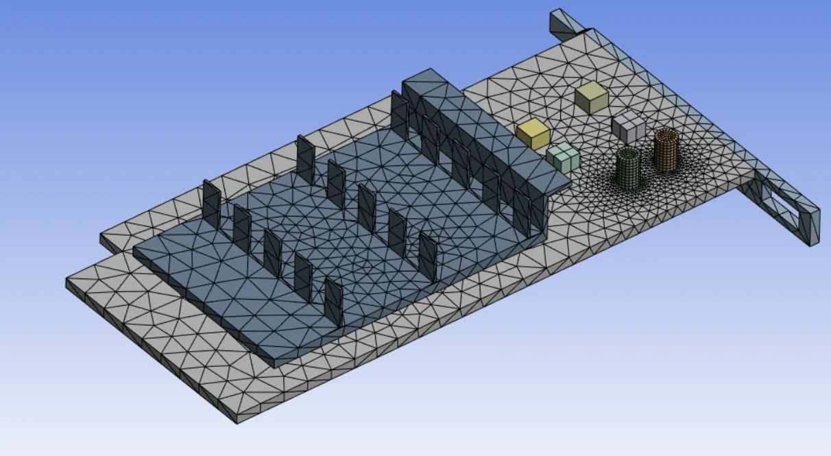Mesh Quality

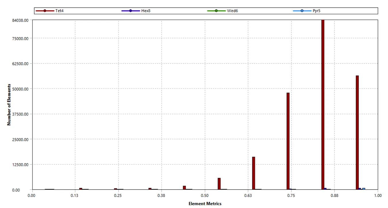
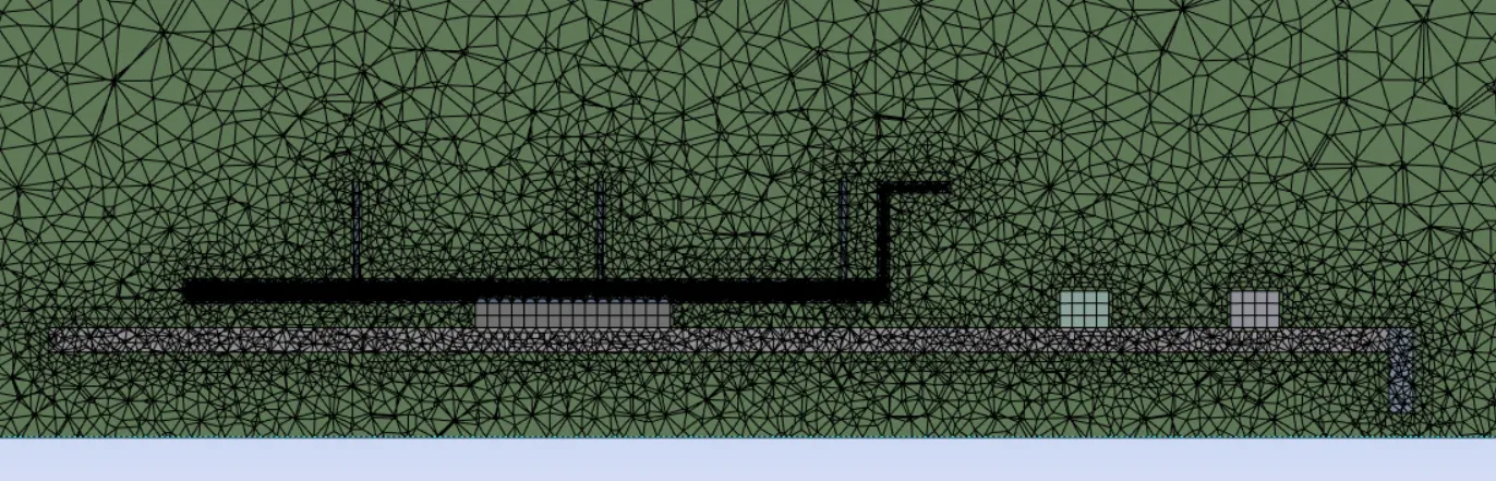
Case2

Overall mesh size 1mm.

Base : Body sizing , element size 0.5mm

Fins : Body sizing , element size 0.1mm

processor : Body sizing , element size 0.5mm

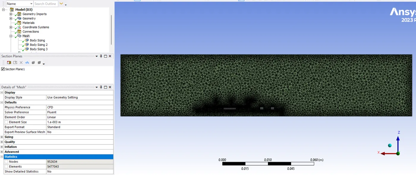
Closer view on Graphics card Assembly

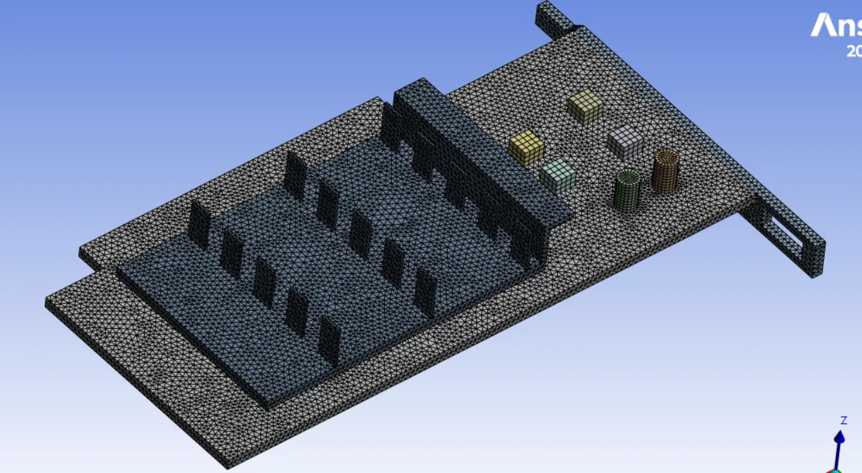
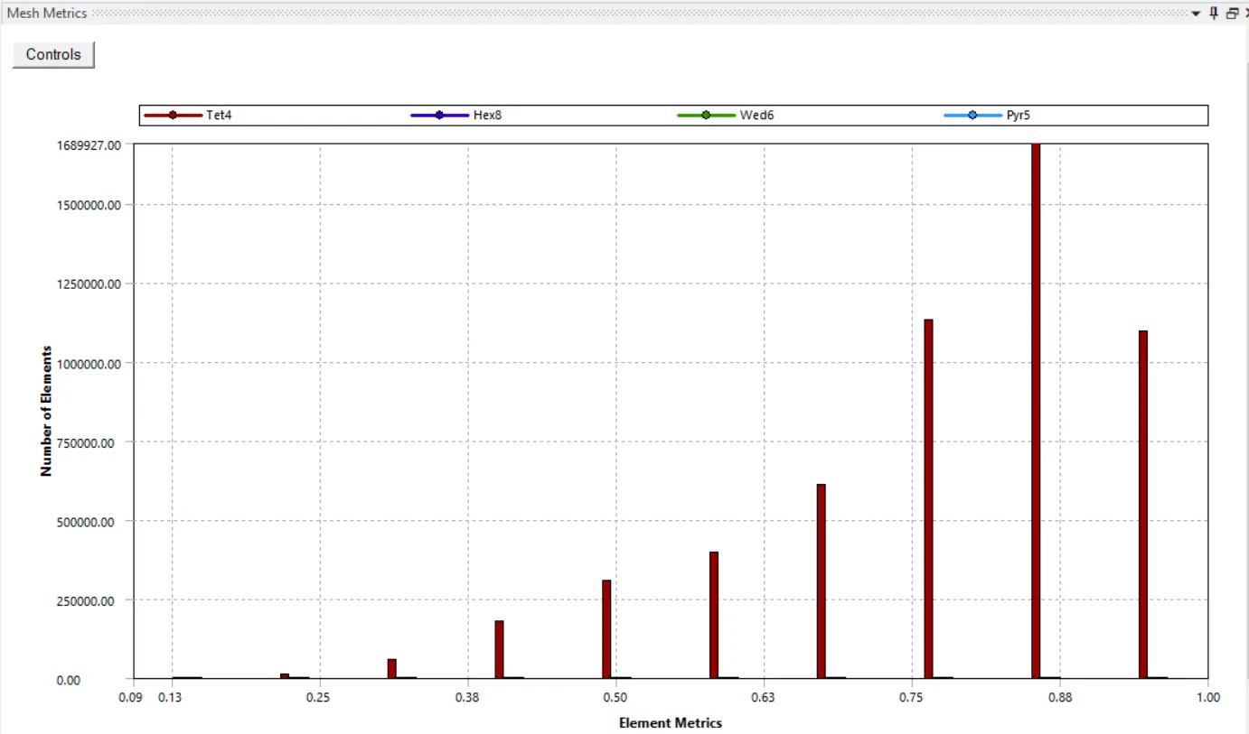
Mesh Quality

Setting up of Physics,

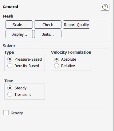
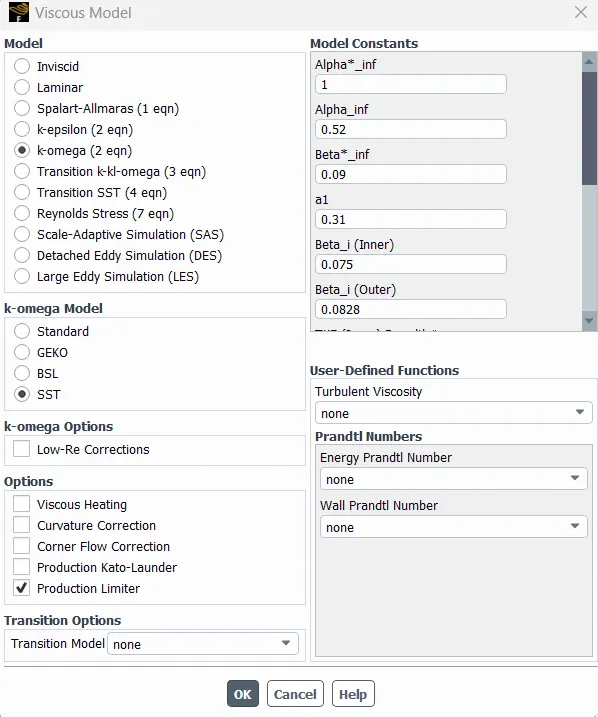
Material Properties

Working fluid

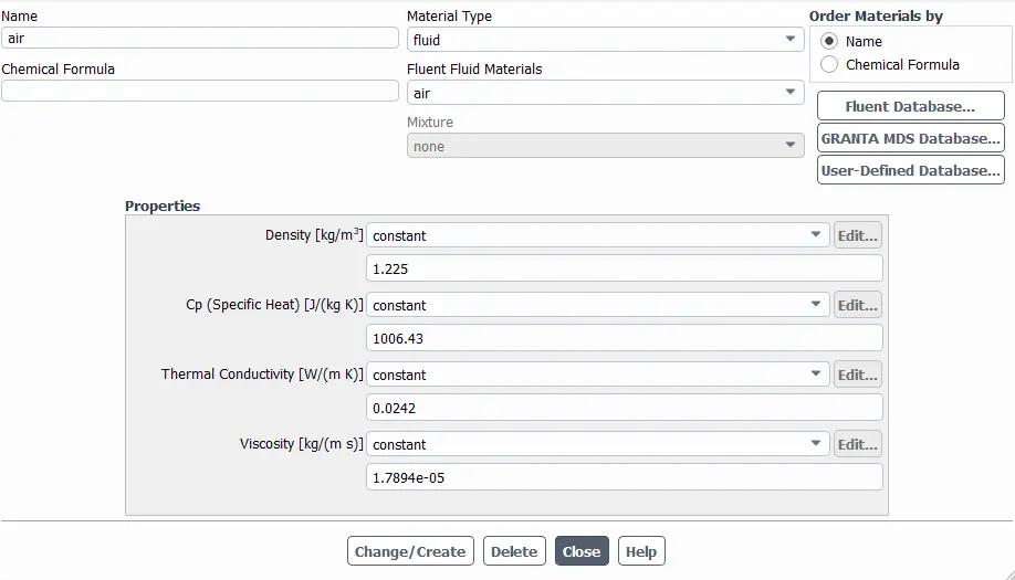
Fins

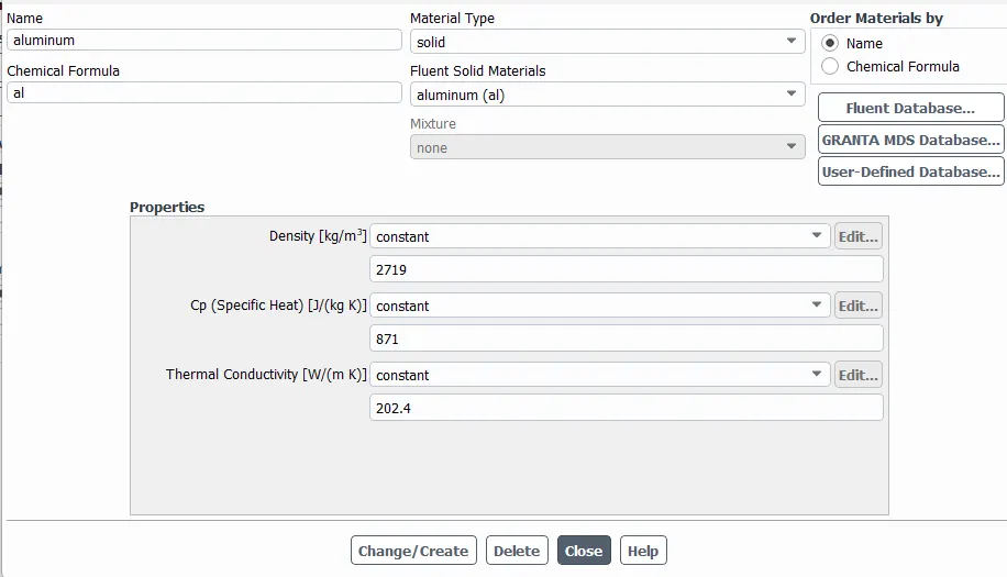
Processor

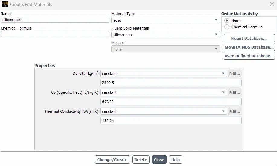
Base Material

Need to assign material to cell zone conditions

Boundary conditions

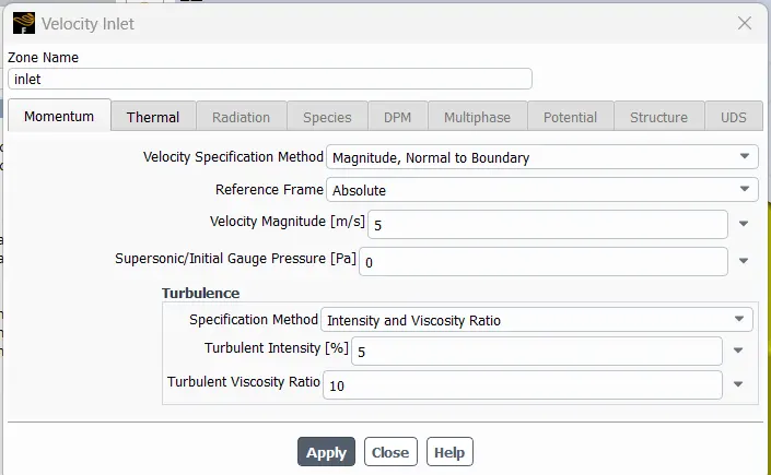
Inlet is considered as velocity input. the velocity 1 m/s, 3 m/s and 5 m/s respectively with each case.

Temperature is 300K

Outlet will be pressure outlet. Gauge pressure is considered zero. Temperature is 300K

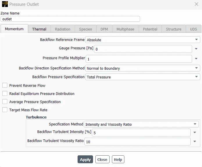
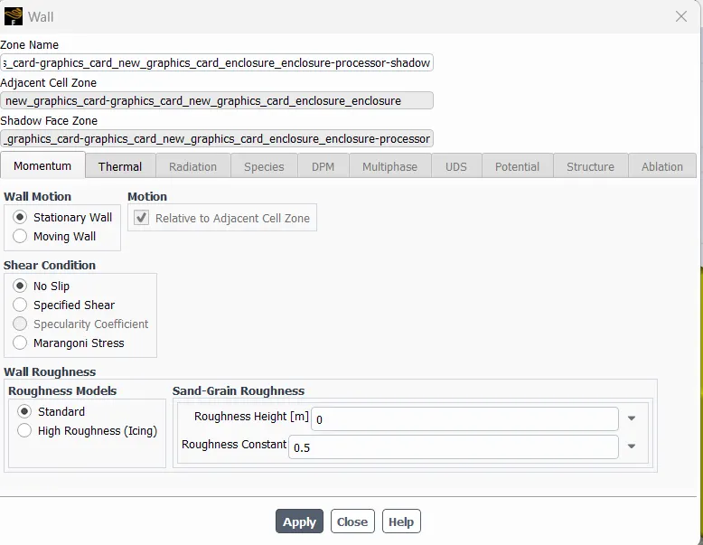
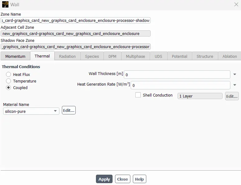
All Other walls are considered stationary and no slip walls condition. Coupled thermal conditions

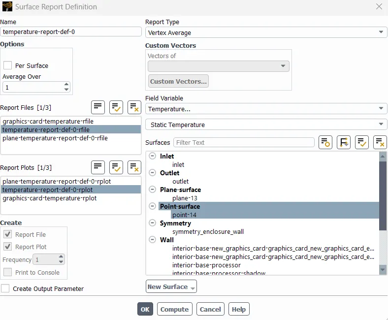
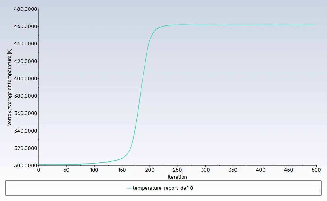
A point inside the processor is used to monitor whether the temperature distribution inside has reached the steady state.

standard Initialization selected.

Analysis of all the cases

Case 1

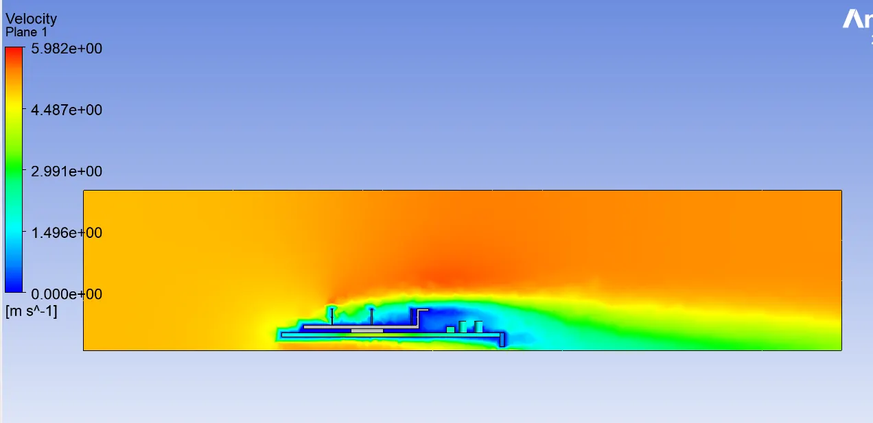
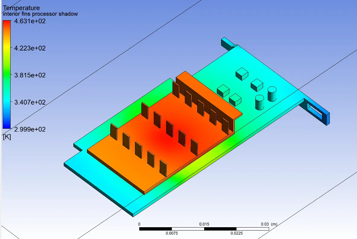
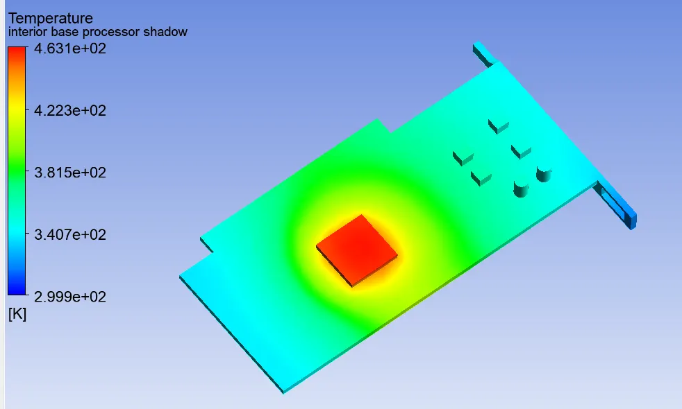
1.1 Description of the case 1

Base Mesh is considered. Inlet velocity is 5m/s.

1.2 Line plot of Residual versus the iteration

1.3 Temperature at monitor point vs iteration (461.5K)

1.4 velocity contour

1.5 Temperature contour

1.6 Temperature Hot spot

Case 2

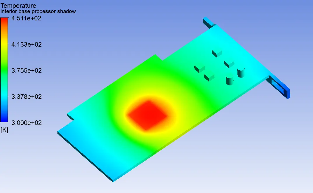
2.1 Description of the case 2

refined Mesh is considered. Inlet velocity is 5m/s.

2.2 Line plot of Residual versus the iteration

2.3 Temperature at monitor point vs iteration (460.5K)

2.4 velocity contour

2.5 velocity contour

2.6 Temperature Hot spot

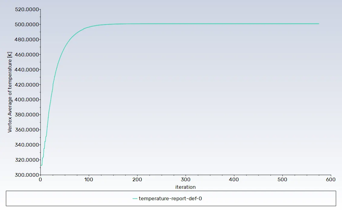
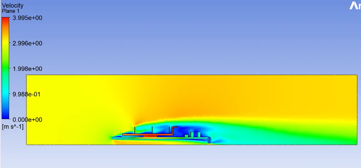
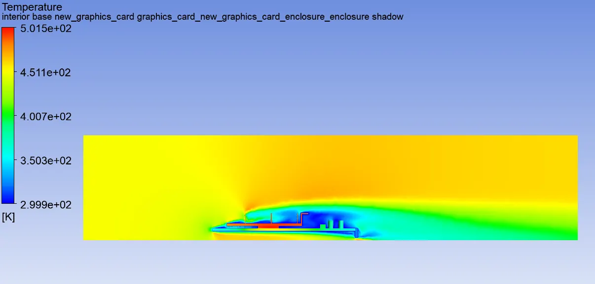
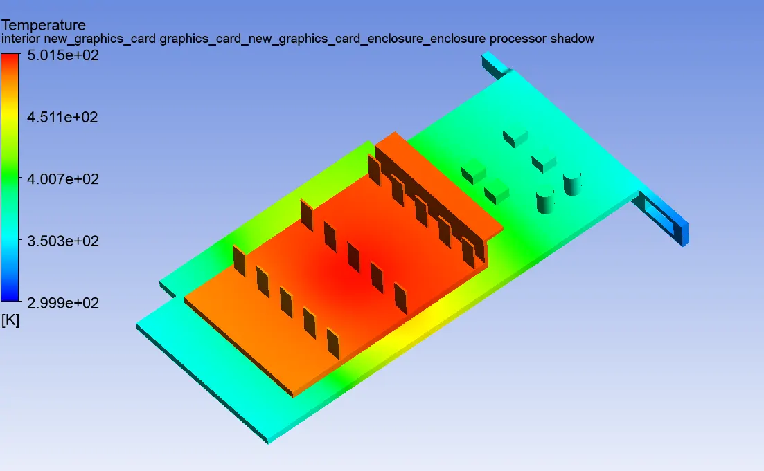
Case 3

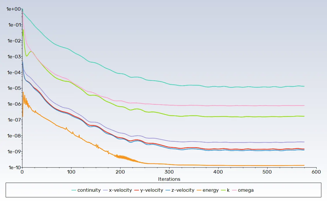
3.1 Description of the case 3

Refined Mesh is considered. Inlet velocity is 3m/s.

3.2 Line plot of Residual versus the iteration

3.3 Temperature at monitor point vs iteration (500.9 K)

3.4 velocity contour

3.5 Temperature contour

3.6 Temperature Hot spot

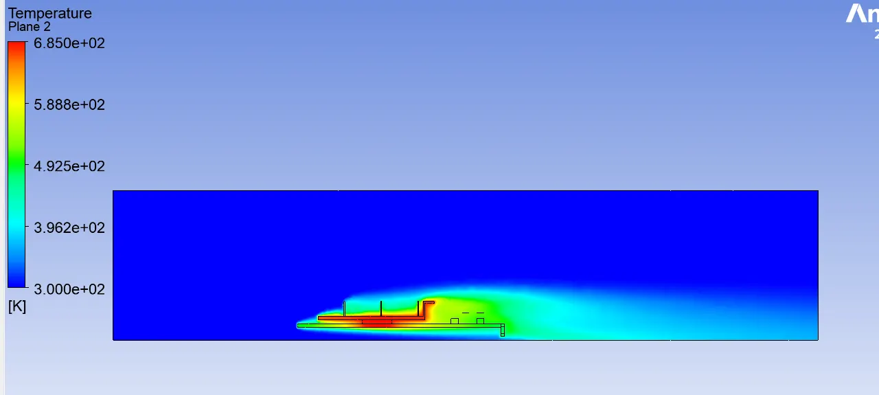
Case 4

4.1 Description of the case 4

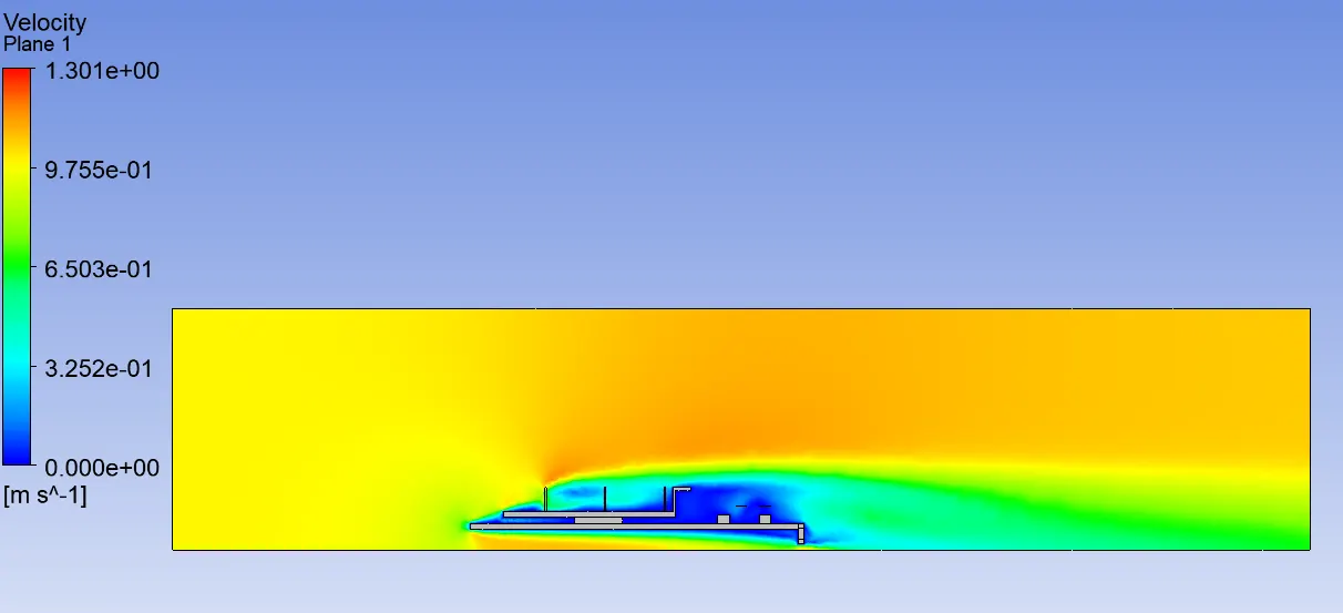
refined Mesh is considered. Inlet velocity is 1m/s.

4.2 Line plot of Residual versus the iteration

4.3 Temperature at monitor point vs iteration (684.5K)

4.4 velocity contour

4.5 Temperature contour

4.6 Temperature Hot spot

Conclusion

Grid Dependence,

By comparing case 1 and case 2

Mesh	No. of cells	Temperature of processor
Base	214410	461.59305
Refined	5477043	460.49713

From the above analysis, we can conclude that the baseline mesh is sufficient to resolve the important flow characteristics and hence we will use the baseline mesh for rest of the study

· As the velocity decreases, we observe that the thermal hot-spots are much stronger in magnitude and have an impact on larger regions of the graphic car. This observation is in line with the theoretical expectation of the effects of the convective heat transfer.