There is a problem in Submitting the challenge so, for better view and detail explanation, Kindly refere PDf Attched.

Aim

· To derive the Derive the following 4th order approximations of the second-order derivative.

1. Central difference

2. Skewed right-sided difference

3. Skewed left-sided difference

· To write a program in Matlab to evaluate the second-order derivative of the analytical function exp(x)*cos(x) and compare it with the 3 numerical approximations that you have derived.

· To provide a plot that compares the absolute error between the above-mentioned schemes

Introduction:

Taylor Series

The Taylor series, named after mathematician Brook Taylor, is a powerful mathematical tool used to approximate functions using polynomials. A special case of the Taylor series occurs when (a = 0). This simplified version is called the Maclaurin series.

Taylor Table method,

The Taylor Table method, also known as the Method of Undetermined Coefficients, is a systematic approach for constructing finite difference schemes with higher-order accuracy. The goal is to create finite difference approximations that meet a desired level of accuracy. By incorporating more terms from the Taylor series expansion than strictly needed, we can express them as finite differences themselves.

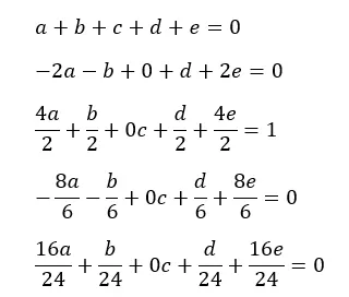
Central difference of 4th order approximations of the second-order derivative

The order of accuracy P = N - Q + 1

Where,

N= Number of nodes in the stencil,

Q= Order of derivative

So we need 5 nodes in stencil to derive the fourth order of second derivative.

Table for central difference

	f(i)	(Δx) f'(x)	(Δx2) f''(x)	(Δx3) f'''(x)	(Δx4) f''''(x)	(Δx5) f'''''(x)
a*f(i-2)	a	-2a	4a/2	-8a/6	16a/24	-32a/120
b*f(i-1)	b	-b	b/2	-b/6	b/24	-b/120
c*f(i)	c	0	0	0	0	0
d*f(i+1)	d	d	d/2	d/6	d/24	d/120
e*f(i+2)	e	2e	4e/2	8e/6	16e/24	32e/120
	0	0	1	0	0	?

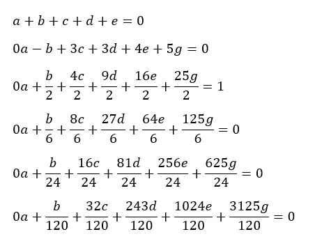
Skewed right sided difference of 4th order approximations of the second-order derivative

The order of accuracy P = N - Q

Where,

N= Number of nodes in the stencil,

Q= Order of derivative

So we need 6 nodes in stencil to derive the fourth order of second derivative.

Table for skewed right sided difference

	f(i)	(Δx) f'(x)	(Δx2) f''(x)	(Δx3) f'''(x)	(Δx4) f''''(x)	(Δx5) f'''''(x)
a*f(i)	a	0	0	0	0	0
b*f(i+1)	b	b	b/2	b/6	b/24	b/120
c*f(i+2)	c	2c	4c/2	8c/6	16c/24	32c/120
d*f(i+3)	d	3d	9d/2	27d/6	81d/24	243d/120
e*f(i+4)	e	4e	16e/2	64e/6	256e/24	1024e/120
g*f(i+5)	g	5g	25g/2	125g/6	625g/24	3125g/120
	0	0	1	0	0	0

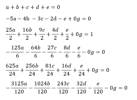
Skewed left sided difference of 4th order approximations of the second-order derivative

The order of accuracy P = N - Q

Where,

N= Number of nodes in the stencil,

Q= Order of derivative

So we need 6 nodes in stencil to derive the fourth order of second derivative.

Table for Skewed left sided difference

	f(i)	(Δx) f'(x)	(Δx2) f''(x)	(Δx3) f'''(x)	(Δx4) f''''(x)	(Δx5) f'''''(x)
a*f(i-5)	a	-5a	25a/2	-125a/6	625a/24	-3125a/120
b*f(i-4)	b	-4b	16b/2	-64b/6	256b/24	-1024b/120
c*f(i-3)	c	-3c	9c/2	-27c/6	81c/24	-243c/120
d*f(i-2)	d	-2d	4d/2	-8d/6	16d/24	-32d/120
e*f(i-1)	e	-e	e/2	-e/6	e/24	-e/120
g*f(i)	g	0	0	0	0	0
	0	0	1	0	0	0

Function

Analytical function f(x) = exp(x)*cos(x)

First Derivative of analytical function f'(x) exp(x)*(cos(x)-sin(x))

Second Derivative of analytical function f'’(x) = -2*exp(x)*(sin(x))

Inputs

x=pi/3;

dx= linspace(pi/4000,pi/2,2000)

Code

The calculation Code

close all
clear all
clc

% analytical function f(x) = exp(x)*cos(x);

% solve the coeffient for central differencing
A=[1,1,1,1,1;
  -2,-1,0,1,2;
  4/2,1/2,0,1/2,4/2;
  -8/6,-1/6,0,1/6,8/6;
 16/24,1/24,0,1/24,16/24;];

B=[0;0;1;0;0;];

%A*X=B
x_c=A\B;

% solve the coeffient for skewed right sided differencing
C=[1,1,1,1,1,1;
    0,1,2,3,4,5;
    0,1/2,4/2,9/2,16/2,25/2;
    0,1/6,8/6,27/6,64/6,125/6;
    0,1/24,16/24,81/24,256/24,625/24;
    0,1/120,32/120,243/120,1024/120,3125/120;];
D=[0;0;1;0;0;0];

%A*X=B
x_r=C\D;

% solve the coeffient for left sided differencing
E=[1,1,1,1,1,1;
    (-5),-4,-3,-2,-1,0;
    25/2,16/2,9/2,4/2,1/2,0;
    -125/6,-64/6,-27/6,-8/6,-1/6,0;
    625/24,256/24,81/24,16/24,1/24,0;
    -3125/120,-1024/120,-243/120,-32/120,-1/120,0;];
F=[0;0;1;0;0;0];

%A*X=B
x_l=E\F;

%inputs
x=pi/3;
dx= linspace(pi/4000,pi/2,2000);


% Analytical Derivative f'(x)= (exp(x)*cos(x)) -(sin(x)*exp(x));
analytical_First_Derivative = exp(x)*(cos(x)-sin(x));

% Analytical second Derivative f"(x)= (exp(x)*cos(x)) -(sin(x)*exp(x));
analytical_second_Derivative = -2*exp(x)*(sin(x));


% fourth_order_central_differencing
% =(af(i-2)+bf(i-1)+cf(i)+df(i+1)+ef(i+2))/dx^2
fourth_order_central_differencing = ((((x_c(1)).*exp(x-2.*dx)).*cos(x-2.*dx))+(((x_c(2)).*exp(x-dx)).*cos(x-dx))+((x_c(3)).*exp(x).*cos(x))+(((x_c(4)).*exp(x+dx).*cos(x+dx)))+(((x_c(5)).*exp(x+2.*dx).*cos(x+2.*dx))))./(dx.^2);


% fourth_order_skewed_right_differencing = af(i)+bf(i+1)+cf(i+2)+df(i+3)+ef(i+4)+gf(i+5))/dx^2
fourth_order_skewed_right_differencing = ((((x_r(1)).*exp(x).*(cos(x)))+((x_r(2)).*exp(x+(1.*dx)).*cos(x+(1.*dx)))+((x_r(3)).*exp(x+(2.*dx)).*cos(x+(2.*dx)))+((x_r(4)).*exp(x+(3.*dx)).*cos(x+(3.*dx)))+((x_r(5)).*exp(x+(4.*dx)).*cos(x+(4.*dx)))+((x_r(6)).*exp(x+(5.*dx)).*cos(x+(5.*dx)))))./(dx).^2;


% fourth_order_skewed_left_differencing = af(i-5)+bf(i-4)+cf(i-3)+df(i-2)+ef(i-1)+gf(i))/dx^2
fourth_order_skewed_left_differencing = (((((x_l(1)).*exp(x-5.*dx).*(cos(x-(5.*dx))))+((x_l(2)).*exp(x-(4.*dx)).*cos(x-(4.*dx)))+((x_l(3)).*exp(x-(3.*dx)).*cos(x-(3.*dx)))+((x_l(4)).*exp(x-(2.*dx)).*cos(x-(2.*dx)))+(((x_l(5)).*exp(x-dx)).*cos(x-dx)))+((x_l(6)).*exp(x).*cos(x))))./((dx).^2);

%error calculation
fourth_order_central_error = abs(analytical_second_Derivative-fourth_order_central_differencing);
fourth_order_skewed_right_error= abs(analytical_second_Derivative-fourth_order_skewed_right_differencing);
fourth_order_skewed_left_error = abs(analytical_second_Derivative-fourth_order_skewed_left_differencing);


% Log plot
figure(1)
loglog (dx,fourth_order_central_error,'m',LineWidth=1);
hold on
loglog(dx,fourth_order_skewed_right_error,'r',LineWidth=1);
hold on
loglog (dx,fourth_order_skewed_left_error,'b',LineWidth=1);

title('The Error log Graph');
ylabel('error')
xlabel('dx')
grid on
legend('central_error','skewed_right_error','skewed_left_error')

% normal plot
figure(2)
plot (dx,fourth_order_central_error,'m',LineWidth=1);
hold on
plot (dx,fourth_order_skewed_right_error,'r',LineWidth=1);
hold on
plot (dx,fourth_order_skewed_left_error,'b',LineWidth=1);
title('The Error Graph plot');
ylabel('error')
xlabel('dx')
grid on
legend('central_error','skewed_right_error','skewed_left_error')


%slope calculation
slope_1=(diff(log(fourth_order_central_error))./diff(log(dx)));
slope_2=(diff(log(fourth_order_skewed_right_error))./diff(log(dx)));
slope_3=(diff(log(fourth_order_skewed_left_error))./diff(log(dx)));


% average of slope

avg_slope_c=mean(slope_1);
avg_slope_r=mean(slope_2);
avg_slope_l=mean(slope_3);



​

Result

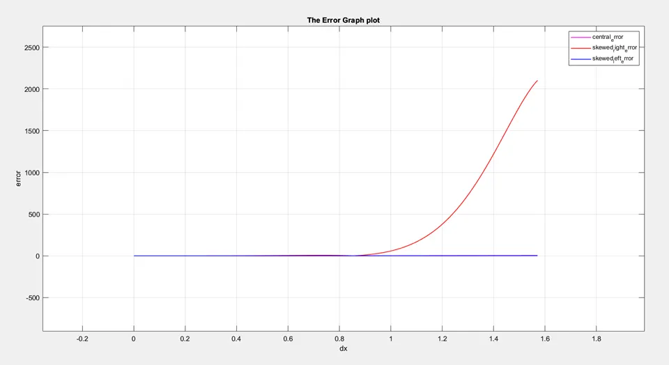
Log plot make more sense than absolute plot.

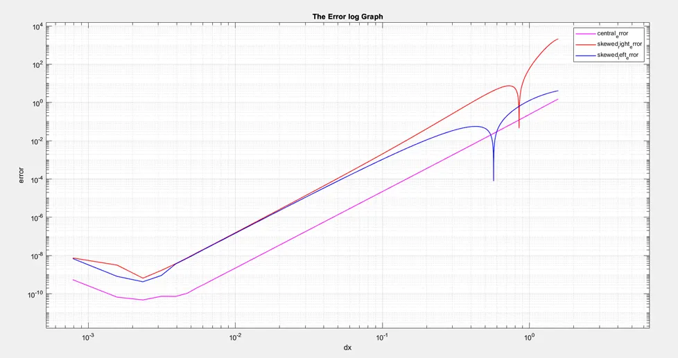
By observing above graph central differencing is more accurate compare to the skewed right and left differencing. The curves will instable when dx is very low and very large. This instability is caused due to the combination of various errors such as roundoff error, residual error and truncation error.

Q. Why skewed scheme is useful? What can a skewed scheme do that a central differencing scheme cannot?

Skewed schemes tend to be more stable in regions with high gradients or strong flow directions Hence the skewed scheme will be useful and we cannot use the central differencing scheme for such an application because it required information from both directions of the point.

Central Differencing Scheme is symmetric and works well for moderate flow gradients. Skewed schemes prioritize stability, while CDS emphasizes accuracy.