Week 1- Mixing Tee
Note: Kindly find the pdf attached with this report for better view
Aim:
-
to find a more suitable model for all the cases among the k-epsilon and k-omega SST model.
-
Compare the Cell count of mesh on the model, Average outlet temperature and Number of iterations for convergence to choose the best one among all the cases.
-
To check the effect on mixing at different pipe lengths.
-
To check the effect on mixing at different moment ratio.
Introduction:
Thermal mixing characterizes the phenomenon where hot and cold flow streams join, mix and result in temperature fluctuations. The temperature fluctuations cause cyclic thermal stresses and subsequent fatigue cracking of the pipe walls.
To decide the strength and life of T-joint pipe its essential to know magnitude of temperature at inlet and outlet, Temperature fluctuation at boundary layer and place where mixing takes place in the pipe and velocity at inlet and outlet.
In this experiment we will find average temperature at outlet surface. Will find the standard deviation at outlet. If the standard deviation more means the mixing considered as not good. The standard deviation should be low as possible to good mixing.
We will find the best model to solve the problem, so we need to compare residual values of the k-epsilon and k-omega SST model. We will also find effectiveness of pipe length and different moment ratio.
The reference formulas as below
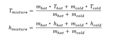
We are using Ansys fluent for preprocessing, solving and post processing. Air used as fluid. mixing of fluids at different temperatures is common within industry such as nuclear power plants, Refrigerator and Air condition equipment.
Physics /Mesh Setup
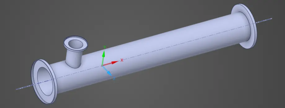
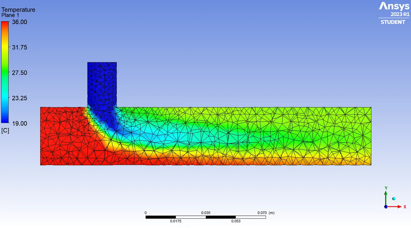
We have used two types of pipes, one longer than the other. The pipe has two inlets and one outlet. The inlet face normal to x axis is called hot inlet where hot fluid enters at 36° Celsius. The inlet face normal to y-axis called Cold inlet where cold fluid enters at 19° Celsius. Hot inlet has bigger diameter compared to cold inlet.
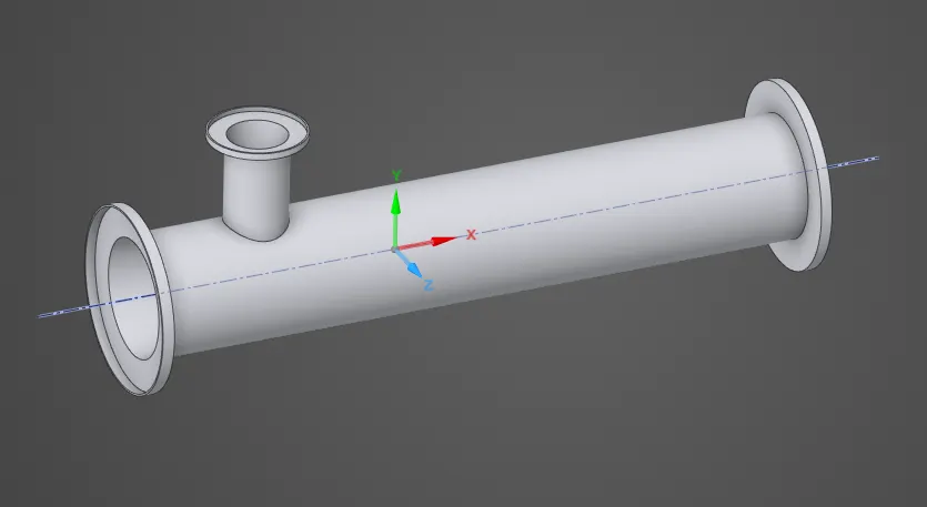
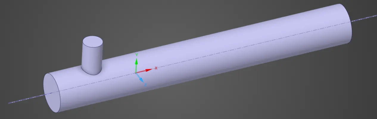
For the Analysis we required only inside volume, so we extracted the desire volume from the pipe by using Ansys Discovery. In the Mesh environment, we will define the Inlet, outlet and wall which helps the Ansys fluent to recognize the parts automatically to solve the problem.
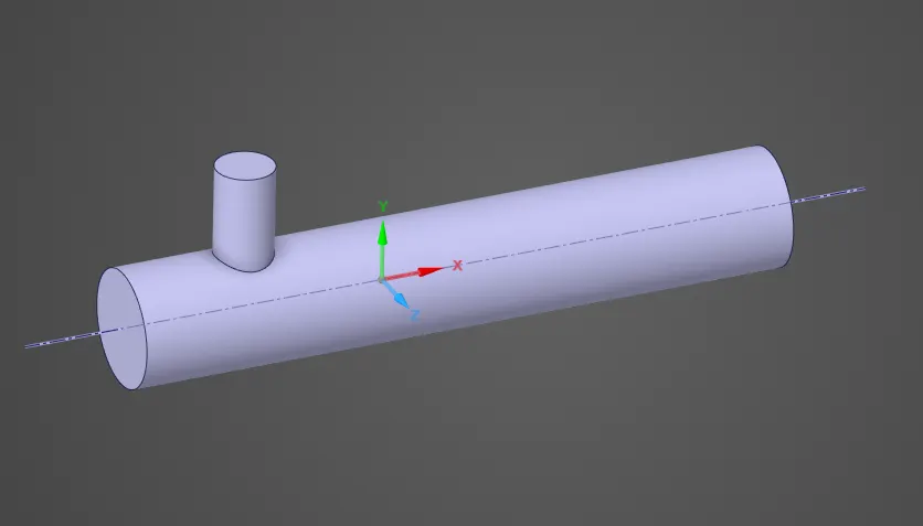
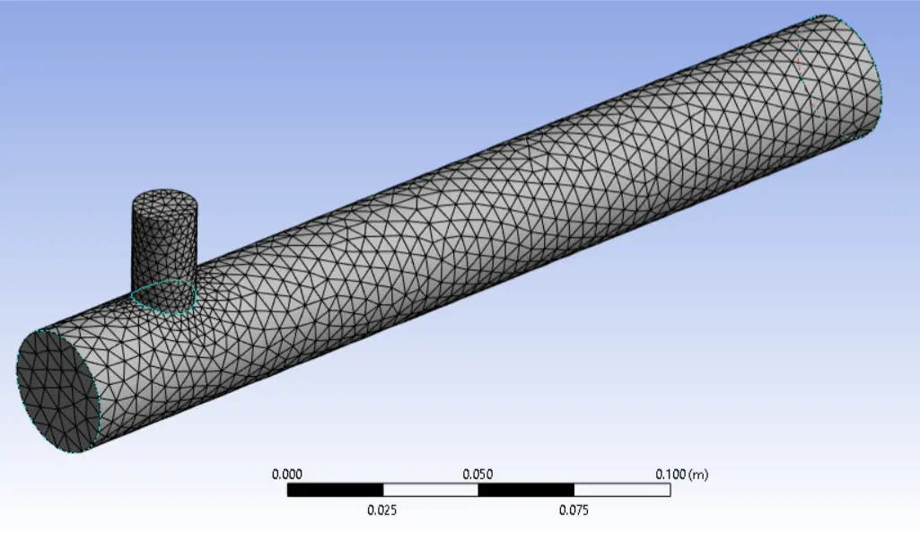
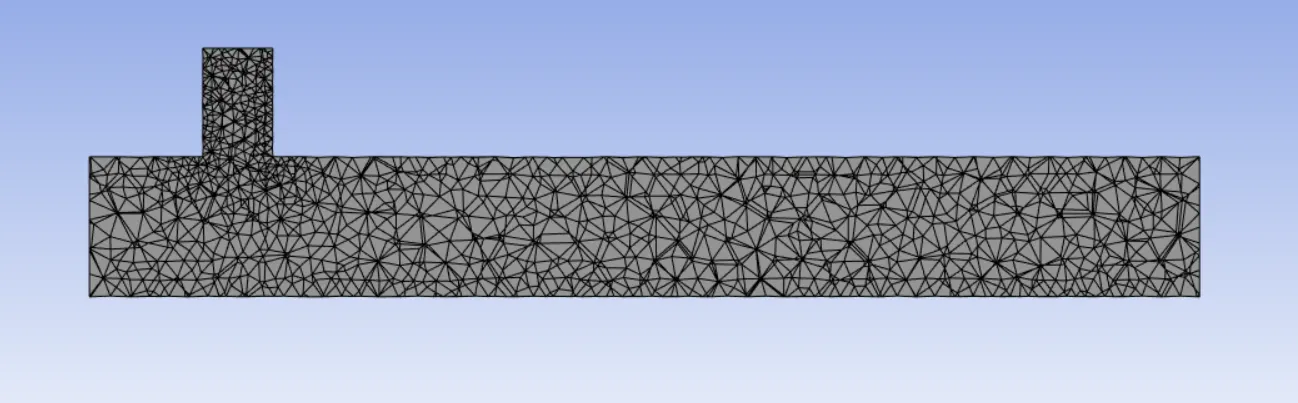
Mesh the model and create middle plane to view mesh quality.
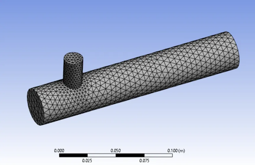
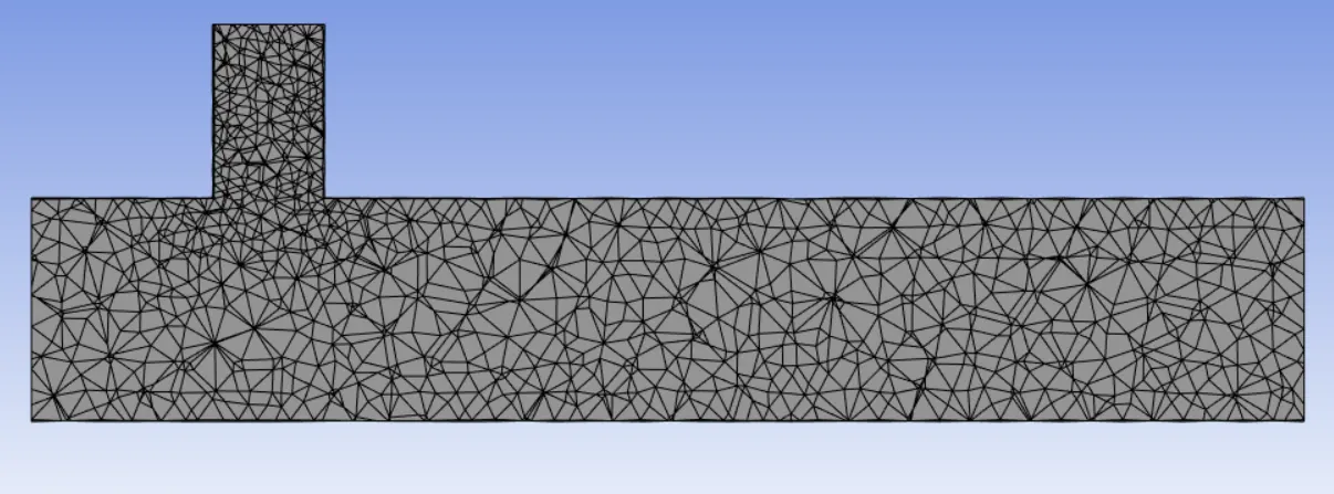
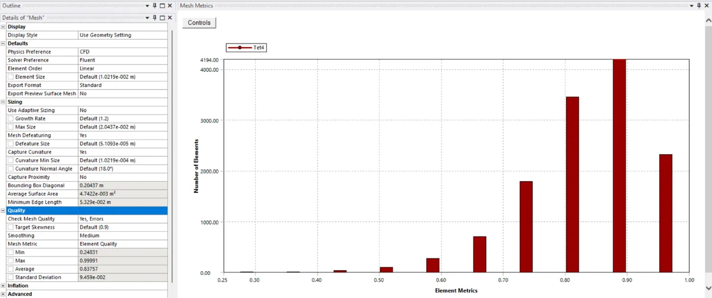
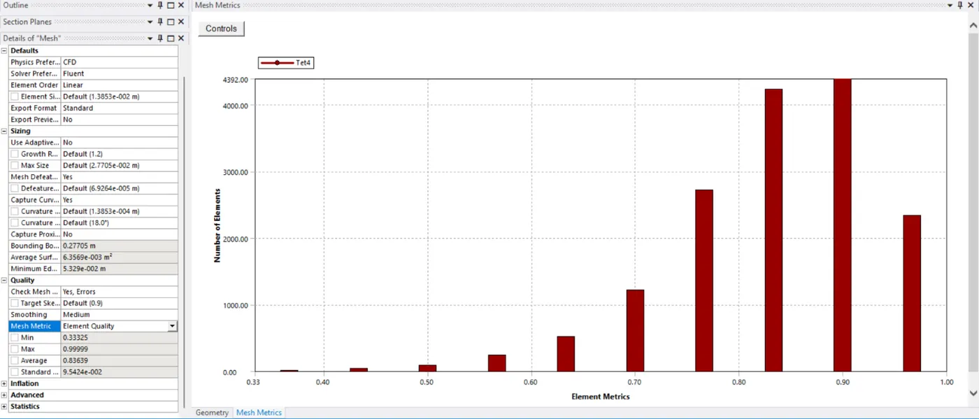
Quality of Mesh elements and elements metrics of short pipe as shown in below picture.
For long pipe,
Mesh, Quality of Mesh elements and elements metrics of long pipe as shown in below picture.
|
Description |
Short Pipe |
Long Pipe |
|
Nodes |
2839 |
3509 |
|
No. of Element |
12804 |
15764 |
|
Element Size |
1.0219e-002 |
1.3853e-002 |
|
Bounding Box Diagonal |
0.20437m |
0.27705m |
Solver Setting
We have used Air as working fluid, so it has low Mach number, selected the pressure-based solver. We are using steady state solver and absolute velocity formation. We are interested in temperature study, so we choose the energy equation too. We have chosen the turbulent model.
We have defined the boundary condition and added the appropriate values. Defined the plot of standard deviation of temperature at outlet. Weighted average velocity and temperature. Initialize the solver with hybrid method. Then calculated with 150 iterations then we continued the calculation till converged.
Analysis of all the cases
Case 1
1.1 Description of the case 1
|
Description |
Values |
|
Pipe Size |
Short |
|
Turbulence model |
K omega SST |
|
Hot Inlet Velocity |
3 m/s |
|
Cold Inlet Velocity |
6 m/s |
|
Temperature at hot inlet |
36°C |
|
Temperature at cold inlet |
19°C |
|
Momentum Ratio |
2 |
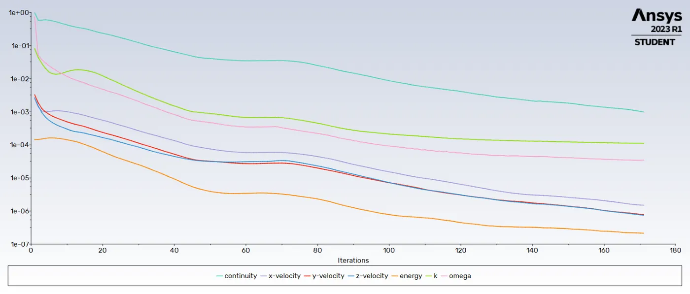
1.2 Line plot of Residual versus the iteration
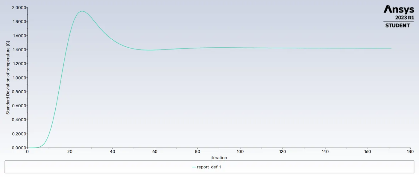
1.3 Line plot of standard deviation temperature versus the iteration
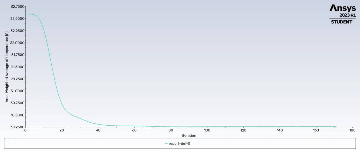
1.4 Line plot temperature versus the iteration
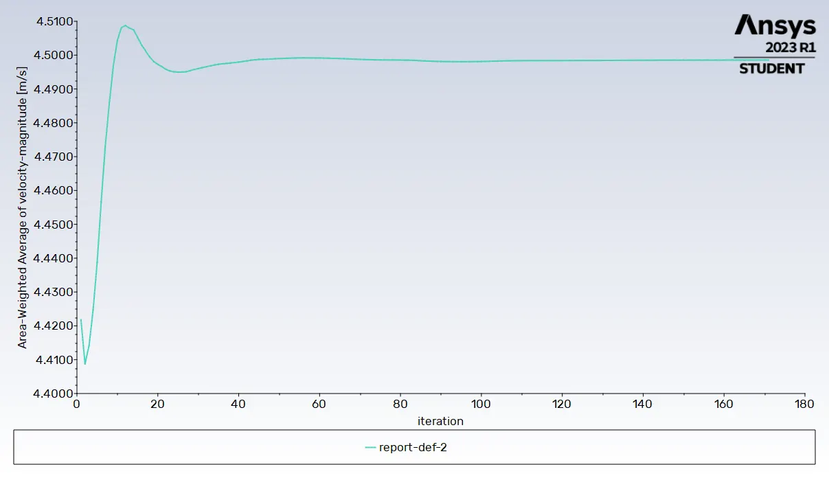
1.5 Line plot Velocity versus the iteration
1.6 Result table
|
Description |
150th Iteration |
Convergence iteration |
|
Convergence iteration |
|
171 |
|
continuity |
1.8272e-03 |
9.9403e-04 |
|
x-velocity |
2.6008e-06 |
1.5027e-06 |
|
y-velocity |
1.4020e-06 |
7.8232e-07 |
|
z-velocity |
1.3850e-06 |
7.4960e-07 |
|
energy |
2.9251e-07 |
2.1415e-07 |
|
k |
1.2356e-04 |
1.1222e-04 |
|
omega |
4.0944e-05 |
3.4528e-05 |
|
Area weighted average of temperature at outlet |
30.2604 |
30.2605 |
|
Standard Deviation of Temperature |
1.4215 |
1.4207 |
|
Area weighted average of Velocity at outlet in m/s |
4.4985 |
4.4986 |
1.7 Temperature contour plot across the pipe
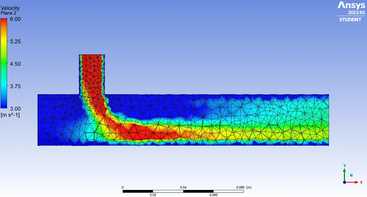
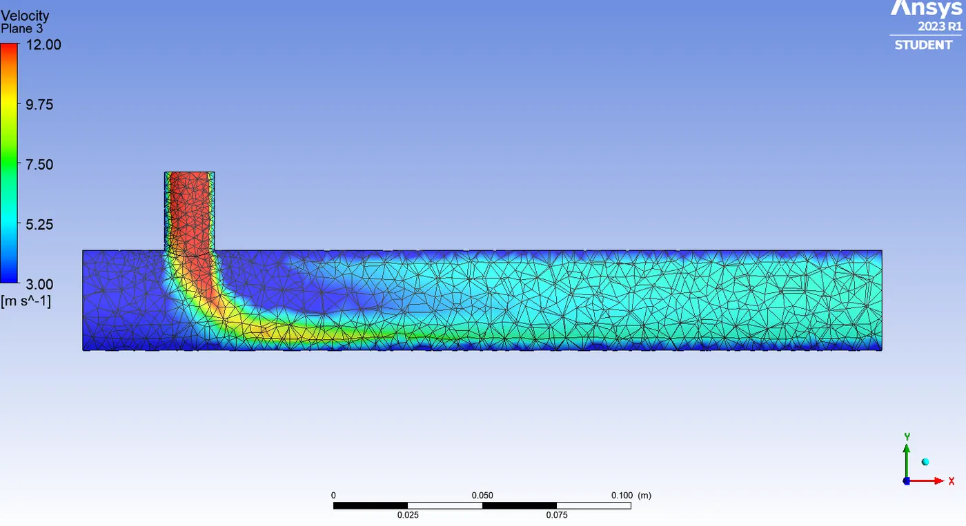
1.8 Velocity contour plot across the pipe
Case 2
2.1 Description of the case 2
|
Description |
Values |
|
Pipe Size |
Short |
|
Turbulence model |
K Epsilon |
|
Hot Inlet Velocity |
3 m/s |
|
Cold Inlet Velocity |
6 m/s |
|
Temperature at hot inlet |
36°C |
|
Temperature at cold inlet |
19°C |
|
Momentum Ratio |
2 |
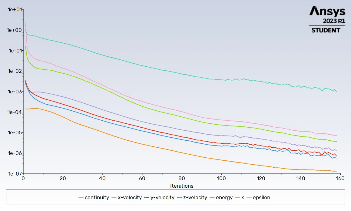
2.2 Line plot of Residual versus the iteration
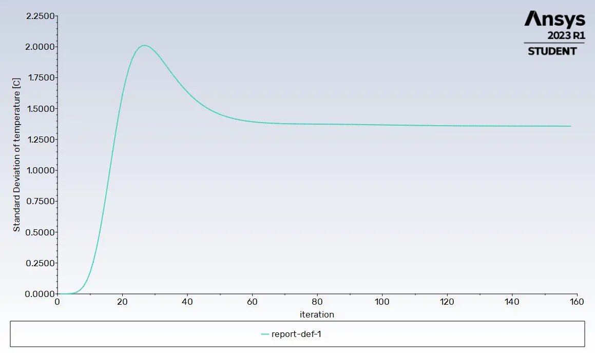
2.3 Line plot of standard deviation temperature versus the iteration
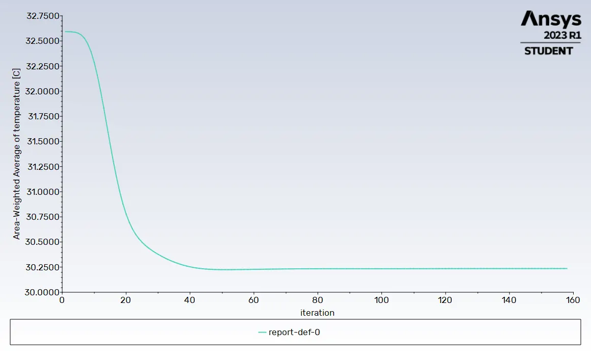
2.4 Line plot temperature versus the iteration
2.5 Line plot Velocity versus the iteration
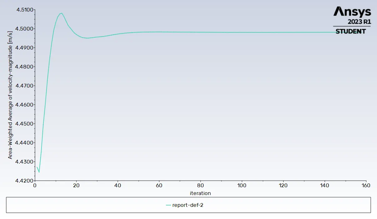
2.6 Result table
|
Description |
150th Iteration |
Convergence iteration |
|
Convergence iteration |
|
158 |
|
continuity |
1.2003e-03 |
9.7421e-04 |
|
x-velocity |
1.8111e-06 |
1.2974e-06 |
|
y-velocity |
8.9715e-07 |
7.2207e-07 |
|
z-velocity |
7.5496e-07 |
5.4771e-07 |
|
energy |
1.4672e-07 |
1.3287e-07 |
|
k |
4.5884e-06 |
3.6553e-06 |
|
omega |
8.7915e-06 |
7.2905e-06 |
|
Area weighted average of temperature at outlet °C |
30.2359 |
30.2360 |
|
Standard Deviation of Temperature °C |
1.3582 |
1.3578 |
|
Area weighted average of Velocity at outlet in m/s |
4.4981 |
4.4981 |
2.7 Temperature contour plot across the pipe
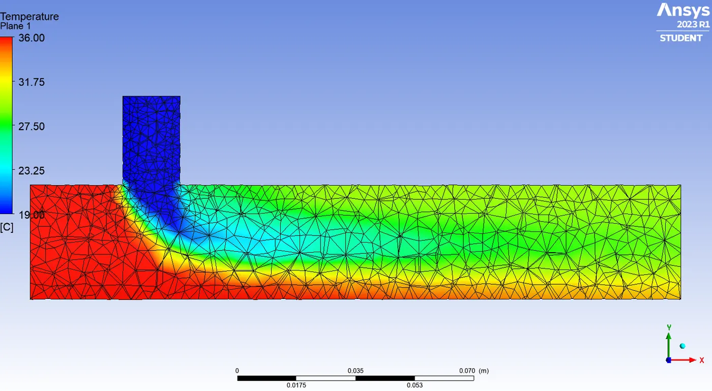
2.8 Velocity contour plot across the pipe
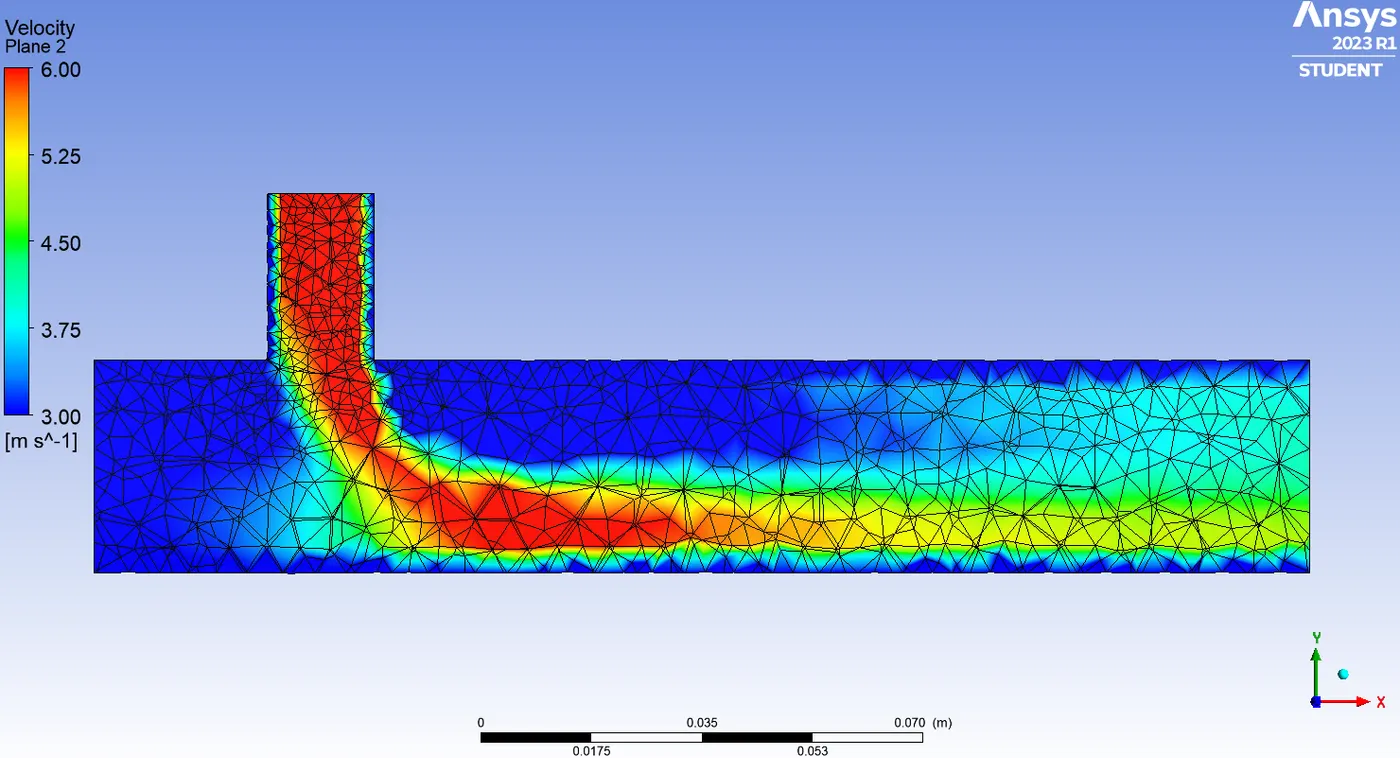
Case 3
3.1 Description of the case 3
|
Description |
Values |
|
Pipe Size |
Short |
|
Turbulence model |
K Epsilon |
|
Hot Inlet Velocity |
3 m/s |
|
Cold Inlet Velocity |
12 m/s |
|
Temperature at hot inlet |
36°C |
|
Temperature at cold inlet |
19°C |
|
Momentum Ratio |
4 |
3.2 Line plot of Residual versus the iteration
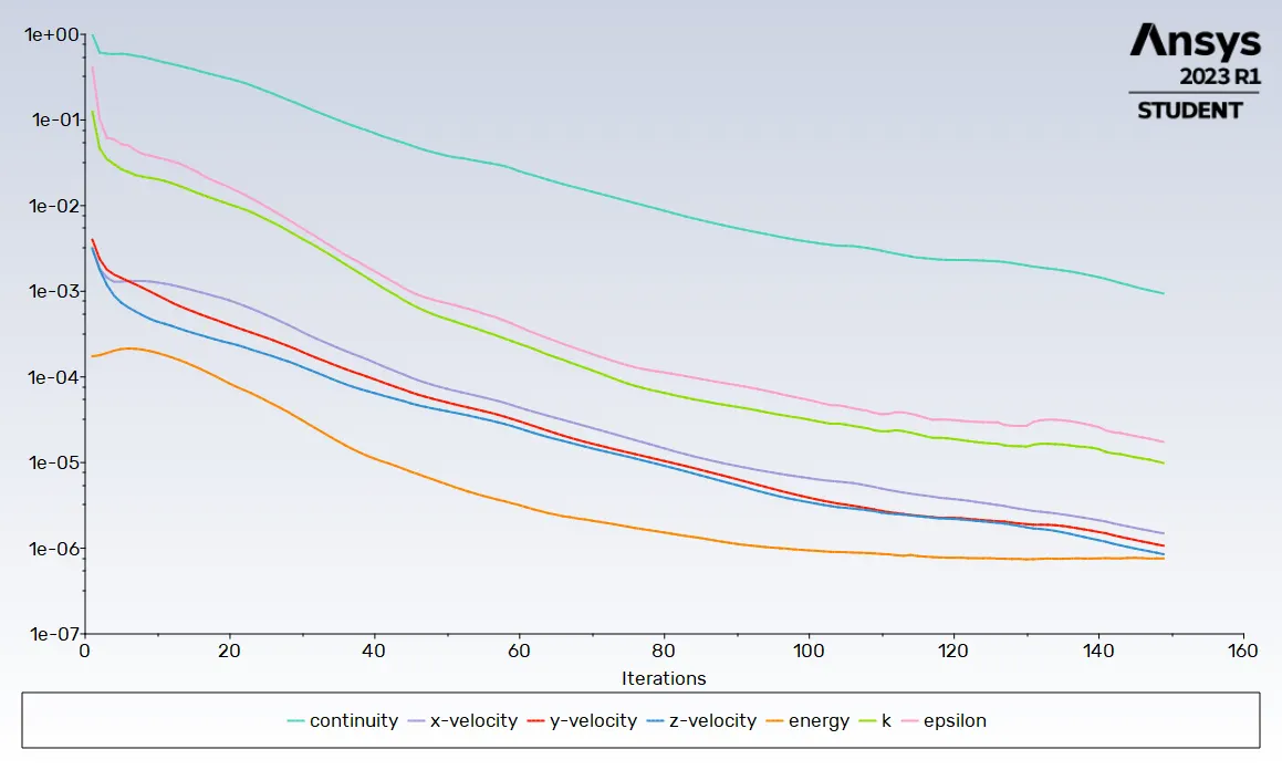
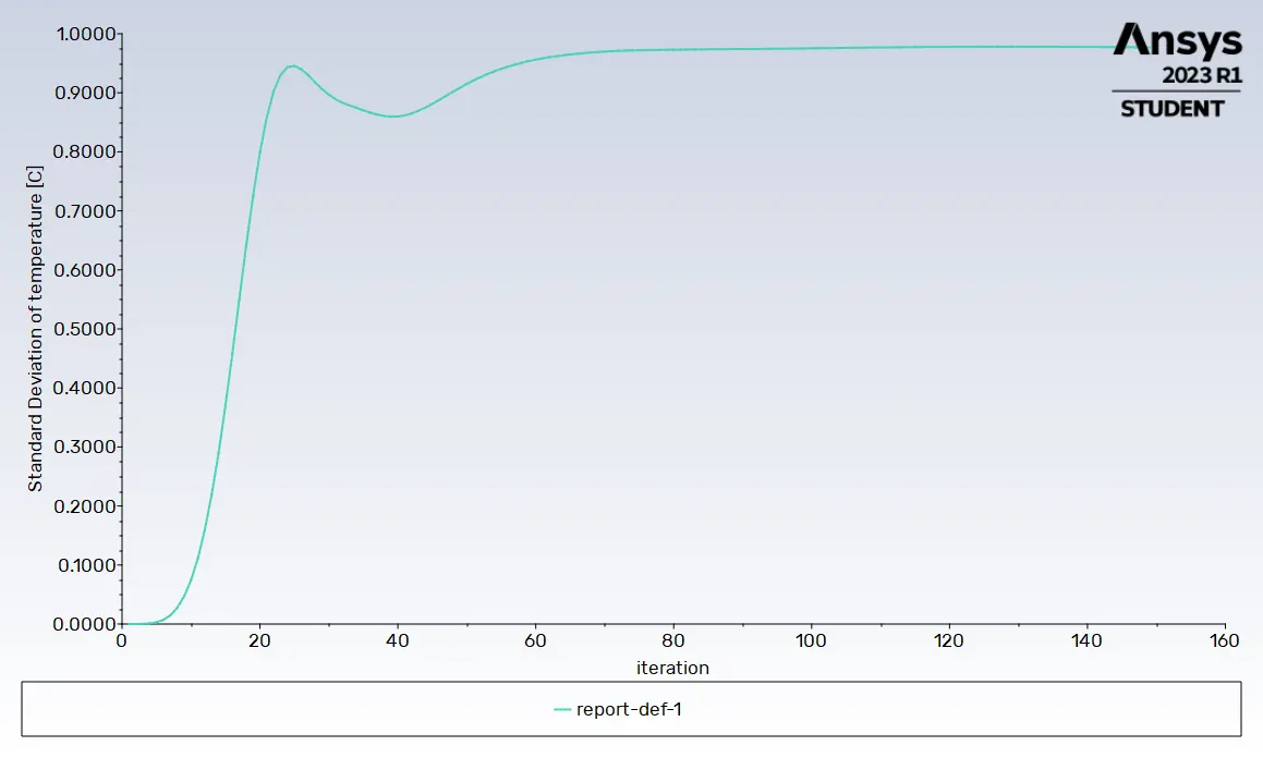
3.3 Line plot of standard deviation temperature versus the iteration
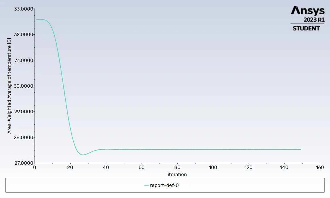
3.4 Line plot temperature versus the iteration
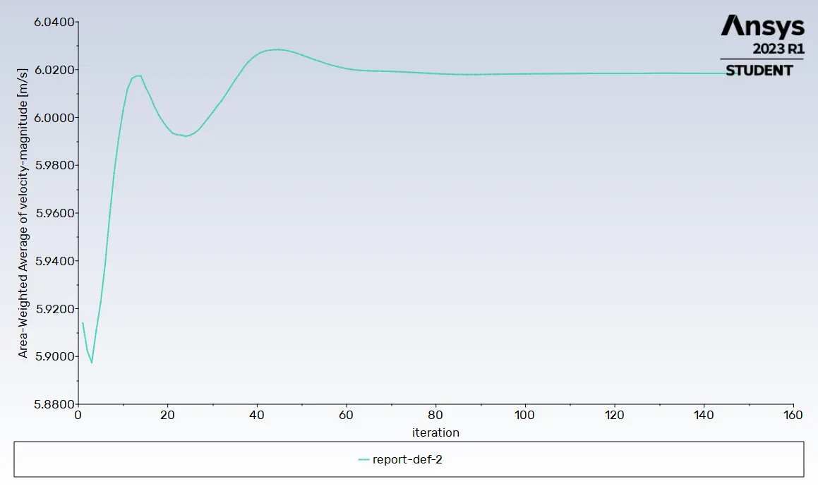
3.5 Line plot Velocity versus the iteration
3.6 Result table
|
Description |
150th Iteration |
Convergence iteration |
|
Convergence iteration |
|
148 |
|
continuity |
|
9.7908e-04 |
|
x-velocity |
|
1.5398e-06 |
|
y-velocity |
|
1.1058e-06 |
|
z-velocity |
|
8.8268e-07 |
|
energy |
|
7.5922e-07 |
|
k |
|
1.0306e-05 |
|
omega |
|
1.8137e-05 |
|
Area weighted average of temperature at outlet |
|
27.5291 |
|
Standard Deviation of Temperature |
|
0.9769 |
|
Area weighted average of Velocity at outlet in m/s |
|
6.0184 |
3.7 Temperature contour plot across the pipe
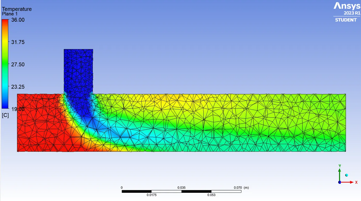
3.8 Velocity contour plot across the pipe
Case 4
4.1 Description of the case 4
|
Description |
Values |
|
Pipe Size |
Long |
|
Turbulence model |
K Epsilon |
|
Hot Inlet Velocity |
3 m/s |
|
Cold Inlet Velocity |
6 m/s |
|
Temperature at hot inlet |
36°C |
|
Temperature at cold inlet |
19°C |
|
Momentum Ratio |
2 |
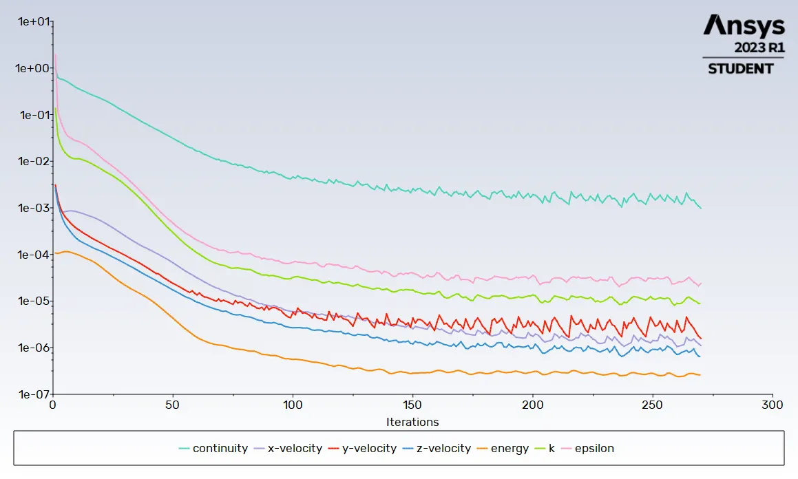
4.2 Line plot of Residual versus the iteration
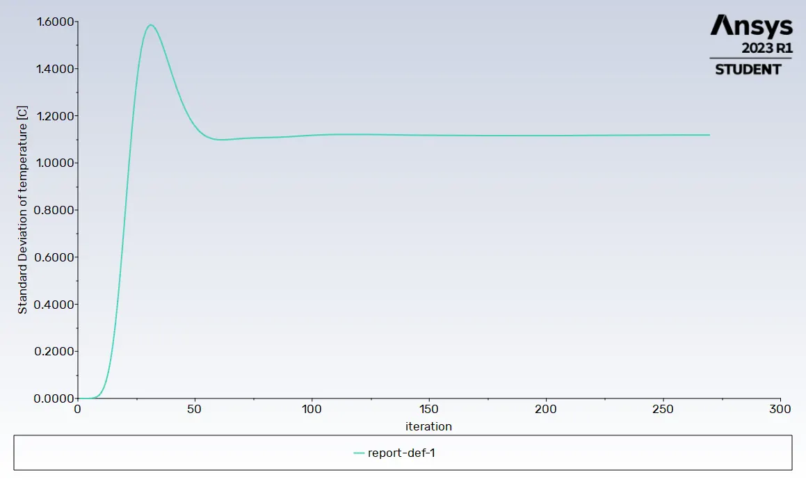
4.3 Line plot of standard deviation temperature versus the iteration
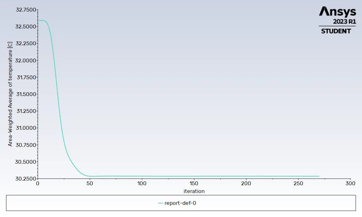
4.4 Line plot temperature versus the iteration
4.5 Line plot Velocity versus the iteration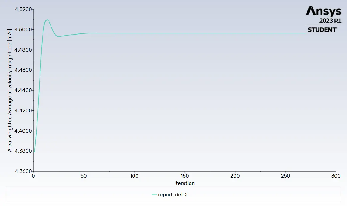
4.6 Result table
|
Description |
150th Iteration |
Convergence iteration |
|
Convergence iteration |
|
270 |
|
continuity |
2.5664e-03 |
9.8395e-04 |
|
x-velocity |
2.5514e-06 |
1.1137e-06 |
|
y-velocity |
4.2786e-06 |
1.5849e-06 |
|
z-velocity |
1.2122e-06 |
6.2890e-07 |
|
energy |
2.8379e-07 |
2.5938e-07 |
|
k |
1.7216e-05 |
8.9728e-06 |
|
omega |
4.0043e-05 |
2.3848e-05 |
|
Area weighted average of temperature at outlet in °C |
30.2861 |
30.2859 |
|
Standard Deviation of Temperature °C |
1.1172 |
1.1185 |
|
Area weighted average of Velocity at outlet in m/s |
4.4964 |
4.4963 |
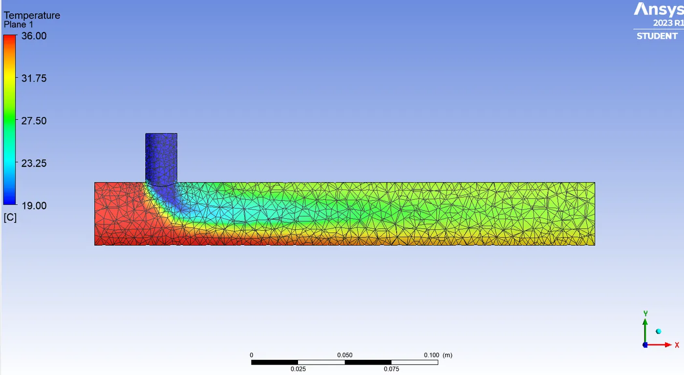
4.7 Temperature contour plot across the pipe
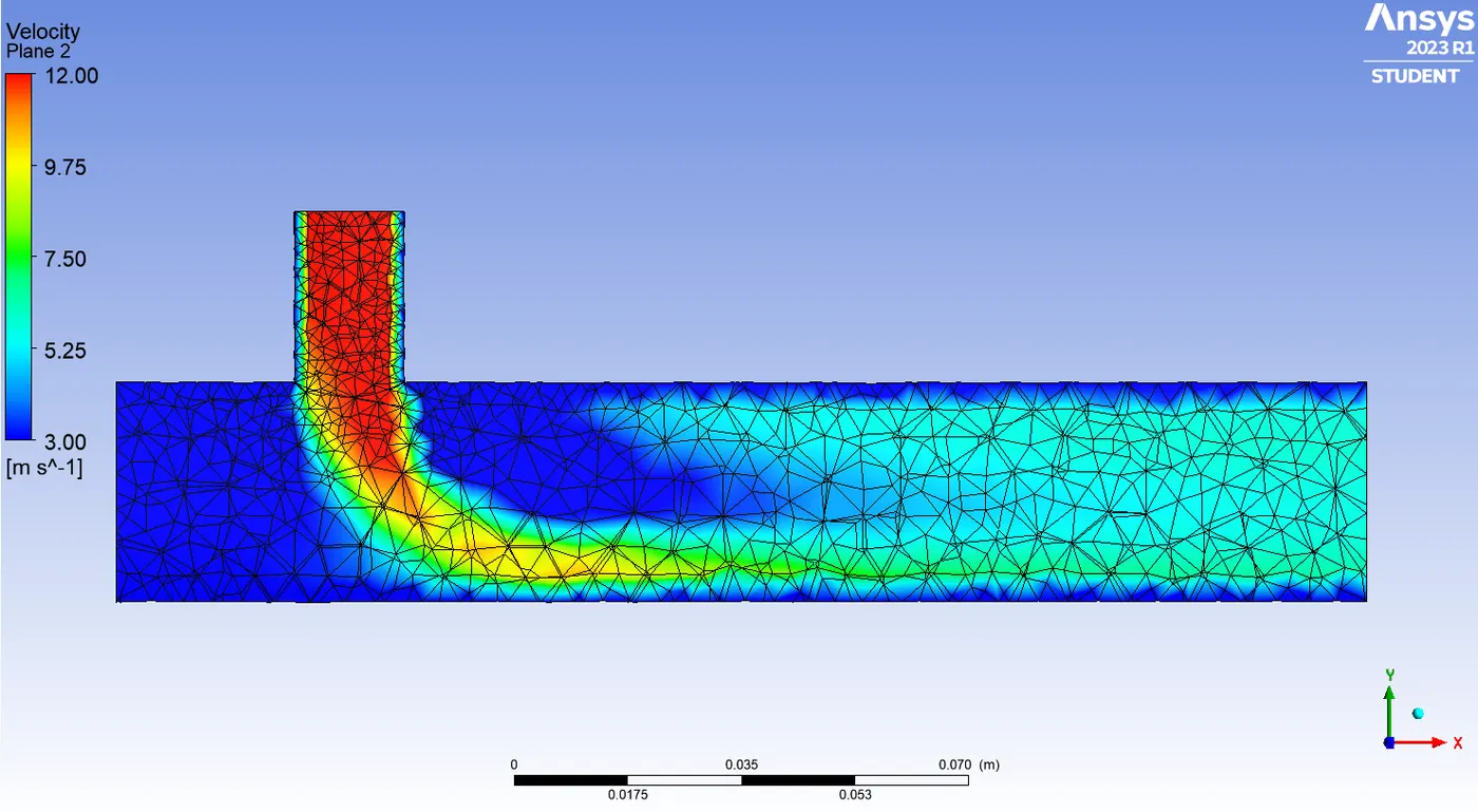
4.8 Velocity contour plot across the pipe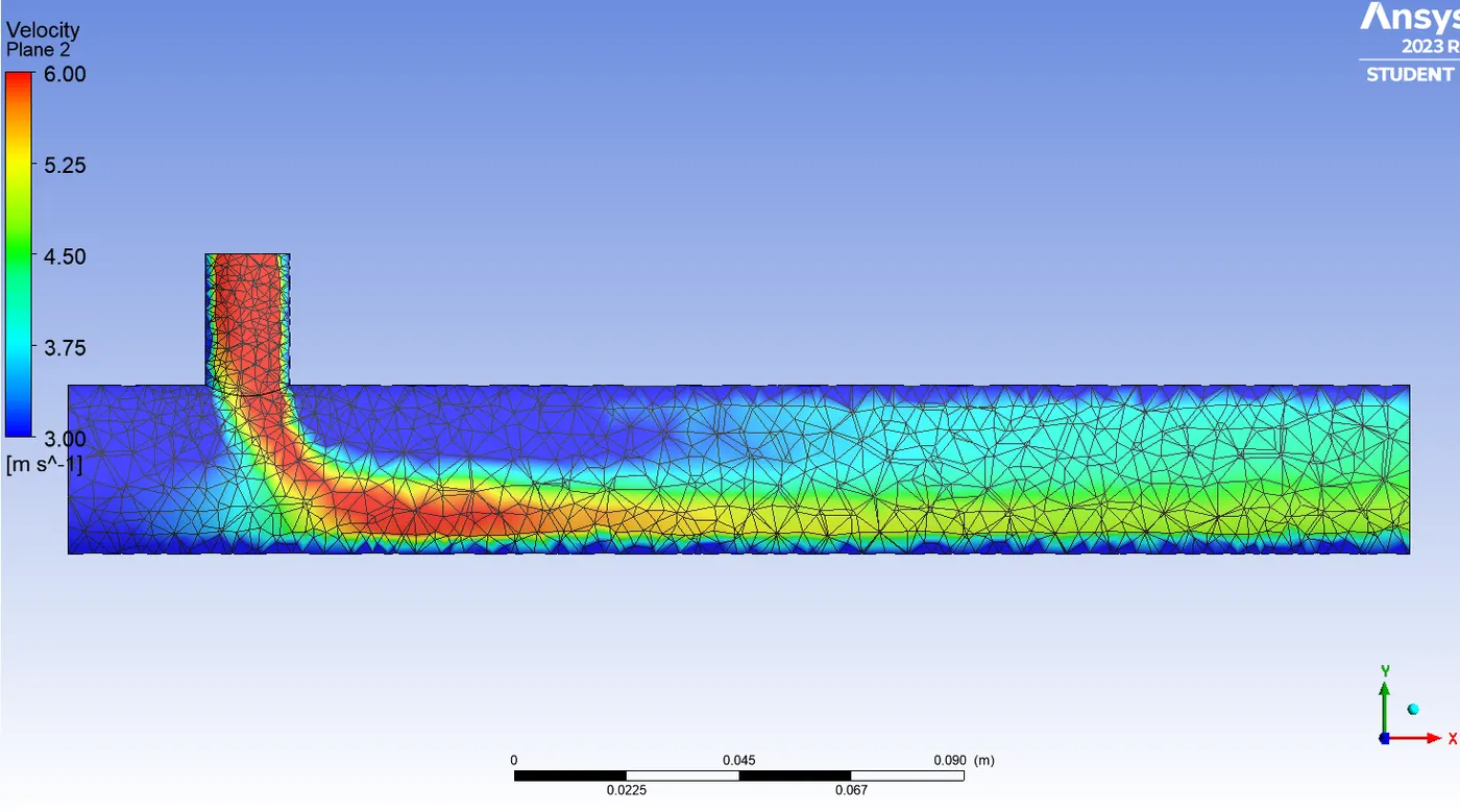
Case 5
5.1 Description of the case 5
|
Description |
Values |
|
Pipe Size |
Long |
|
Turbulence model |
K Epsilon |
|
Hot Inlet Velocity |
3 m/s |
|
Cold Inlet Velocity |
12 m/s |
|
Temperature at hot inlet |
36°C |
|
Temperature at cold inlet |
19°C |
|
Momentum Ratio |
4 |
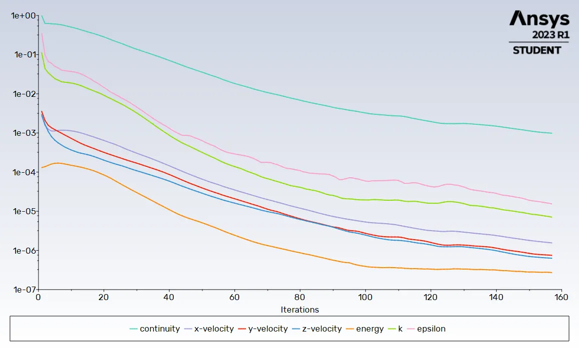
5.2 Line plot of Residual versus the iteration
5.3 Line plot of standard deviation temperature versus the iteration
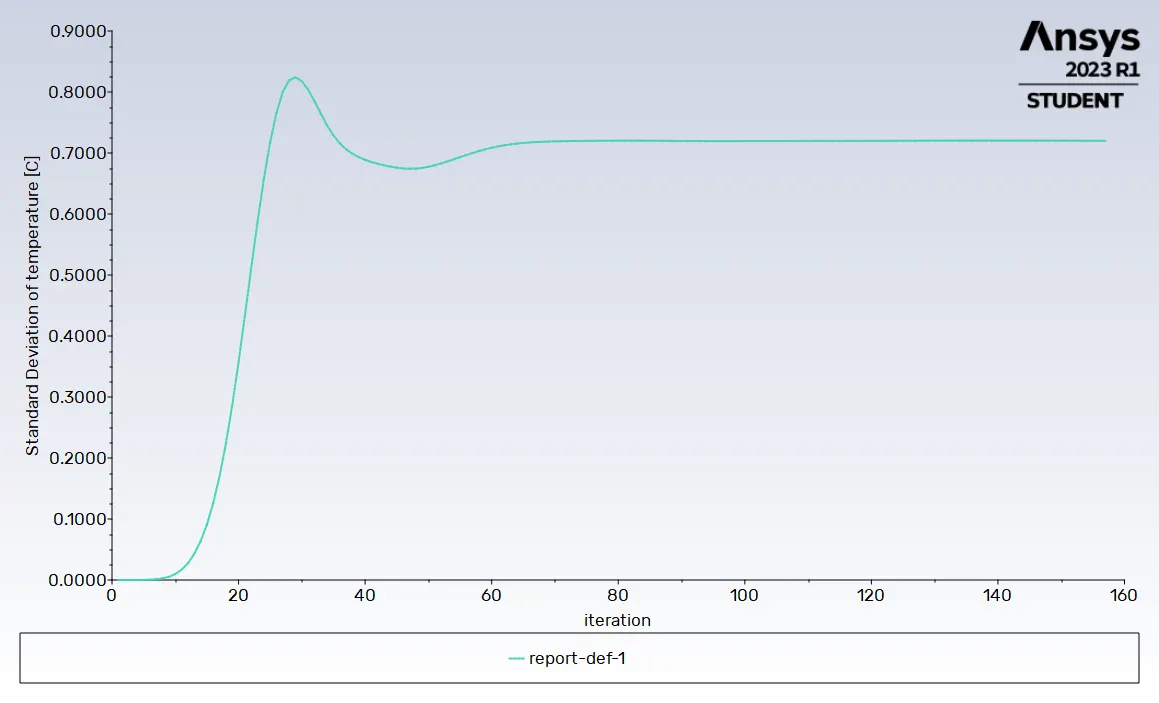
5.4 Line plot temperature versus the iteration
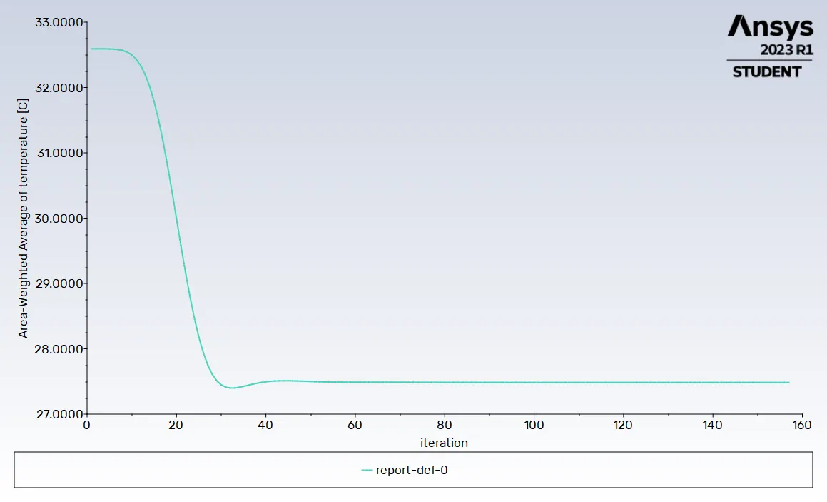
5.5 Line plot Velocity versus the iteration
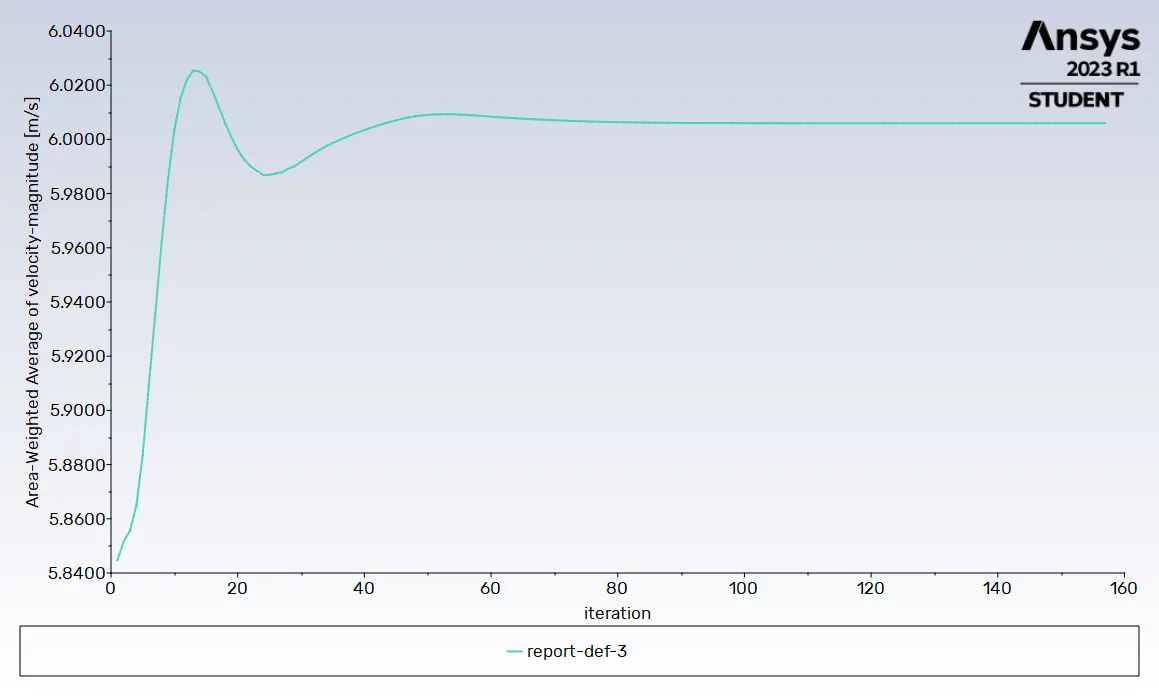
5.6 Result table
|
Description |
150th Iteration |
Convergence iteration |
|
Convergence iteration |
|
157 |
|
continuity |
1.1350e-03 |
9.8531e-04 |
|
x-velocity |
1.8055e-06 |
1.5563e-06 |
|
y-velocity |
8.4289e-07 |
7.4842e-07 |
|
z-velocity |
7.0172e-07 |
6.3094e-07 |
|
energy |
2.8043e-07 |
2.7188e-07 |
|
k |
8.6480e-06 |
7.0913e-06 |
|
omega |
1.9115e-05 |
1.5411e-05 |
|
Area weighted average of temperature at outlet in °C |
27.4843 |
27.4841 |
|
Standard Deviation of Temperature °C |
0.7202 |
0.7200 |
|
Area weighted average of Velocity at outlet in m/s |
6.0060 |
6.0060 |
5.7 Temperature contour plot across the pipe
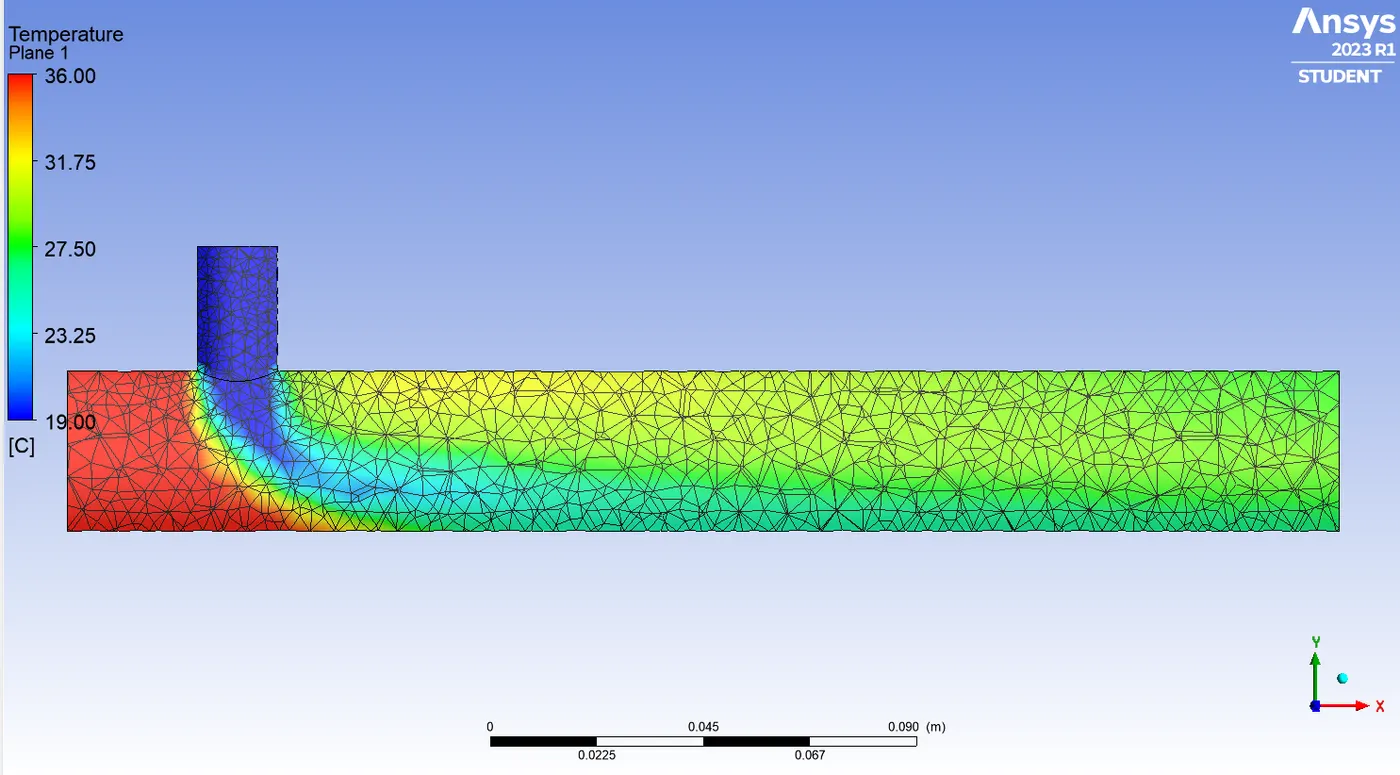
5.8 Velocity contour plot across the pipe
Conclusion
1. Comparing K- omega and k-Epsilon Turbulent model
By comparing result table of case 1 and case 2 (1.6 & 2.6),
|
Description |
K-Omega SST |
K-Epsilon |
|
Convergence iteration |
171 |
158 |
|
Standard Deviation of temperature |
1.4207 |
1.3578 |
|
Residual Values |
Higher |
Lower |
We have chosen K- epsilon turbulence model over K-omega SST because,
-
Taking longer time to converge
-
The lesser the standard deviation, the higher the mixing quality. As per the above table standard deviation of temperature at outlet is higher for K-omega SST.
-
All the residual values are lesser for K-epsilon compared to K-omega so accuracy will be more in K-epsilon.
2. Comparision of different Cases
|
Description |
Short mixing Tee, Moment ratio 2 Case2 |
Short mixing Tee, Moment ratio 4 Case3 |
Long mixing Tee, Moment ratio 2 Case 4 |
Long mixing Tee, Moment ratio 4 Case5 |
|
Cell Count |
12804 |
12804 |
15764 |
15764 |
|
Average outlet temperature °C |
30.2360 |
27.5291 |
30.2859 |
27.4841 |
|
Number of iterations to convergence |
158 |
148 |
270 |
157 |
|
Average Velocity at outlet in m/s |
4.4981 |
6.0184 |
4.4963 |
6.0060 |
3.Effect of length and momentum ratio
As per the above comparison table, length of the pipe doesn't affect the mixing. The difference between the outlet temperature of long and short pipe is negligible, that is approximately 0.05°C.
The momentum ratio of the fluid affects the mixing process. The higher the momentum ratio, the better the mixing process.