Week 2 - Flow over a Cylinder.
Aim:
· explain the phenomenon of Karman vortex street.
· Simulate the flow with the steady and unsteady case and calculate the Strouhal Number for Re= 100.
· Calculate the coefficient of drag and lift over a cylinder by setting the Reynolds number to 10,100,1000,10000 & 100000. (Run with steady solver)
· Discuss the effect of Reynolds number on the coefficient of drag. [ Results should be validated with any standard literature and error should be within 5 %]
· Plots of the coefficient of drag and lift.
· Plots to show vortex shedding behind the cylinder.
Introduction:
A Kármán vortex street is a repeating pattern of swirling vortices that appear in the wake of an obstacle in a fluid, caused by a process known as vortex shedding. This phenomenon is responsible for the unsteady separation of flow of a fluid around blunt body. It is named after the engineer and fluid dynamicity Theodore von Kármán.
The Kármán vortex street is responsible for such phenomena as the “singing” of suspended telephone or power lines and the vibration of a car antenna at certain speeds. Mathematical modelling of von Kármán vortex street can be performed using different techniques including but not limited to solving the full Navier-Stokes equations with k-epsilon, SST, k-omega and Reynolds stress, and large eddy simulation (LES) turbulence models.
A vortex street forms only at a certain range of flow velocities, specified by a range of Reynolds numbers (Re), typically above a limiting Re value of about 90.
In urban areas where there are many other tall structures nearby, the turbulence produced by these can prevent the formation of coherent vortices. Periodic crosswind forces set up by vortices along object's sides can be highly undesirable, due to the vortex-induced vibrations caused, which can damage the structure, hence it is important for engineers to account for the possible effects of vortex shedding when designing a wide range of structures, from submarine periscopes to industrial chimneys and skyscrapers.
This formula generally holds true for the range 250 < Red < 200000:
St=0.198(1−19.7Re�)
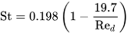

where:St=���
· f = vortex shedding frequency.
· d = diameter of the cylinder (characteristic length)
· U = flow velocity.
This dimensionless parameter St is known as the Strouhal number.
The Strouhal number is a dimensionless number describing oscillating flow mechanisms. The Strouhal number represents the ratio of inertial forces due to the local acceleration of the flow to the inertial forces due to the convective acceleration. Depending on the time scale of the problem, this ratio may be of order unity, and therefore its importance is not obvious.
In flows characterized by a periodic motion, the Strouhal number is associated with the oscillations of the flow due to the inertial forces relative to the changes in velocity due to the convective acceleration of the flow field.
For very small Reynolds numbers, the flow is completely laminar around the cylinder, with no recirculation and no instability.
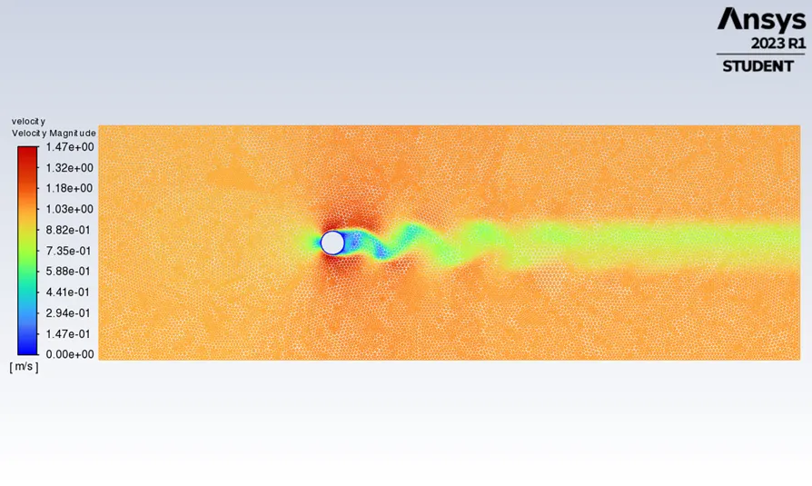
For larger Reynolds numbers, a recirculation zone appears behind the obstacle. More precisely, two eddies with opposite signs appear just behind the cylinder and remain close to it.
For larger Reynolds numbers, these eddies are unstable and successively leave the cylinder to propagate in the wake, to form the so called “Von Karman” vortex street.
Physics /Mesh Setup
We have rectangle computational domain. We are using symmetry boundary condition 60m and 20m apart. We have placed cylinder of diameter(D) 2, which is place 20m that is 10D away from velocity inlet and 10m that is 5D from the top boundary.
|
|
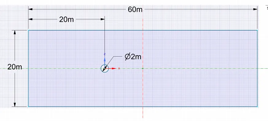
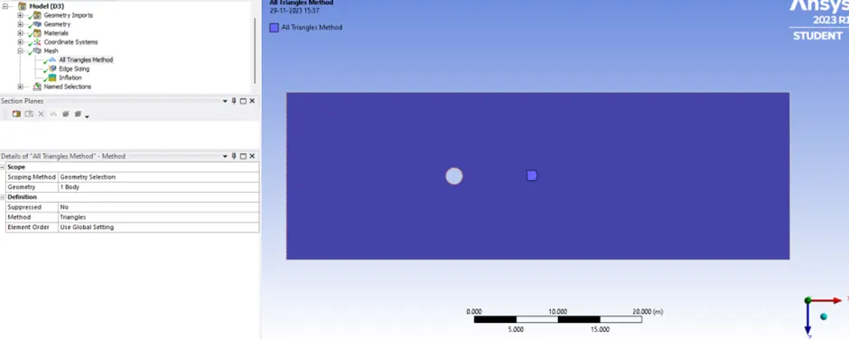
Mesh the model and view mesh quality. To improve the mesh, we are adding different methods to the mesh. First one is automatic mesh and we select the whole surface and select the triangle method. Update the mesh.
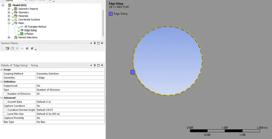
Add sizing method to the cylinder/circle. Select the edge of circle. Select the number of divisions to 36.
Add inflation layer to circle. Inflation layer helps create body fitted mesh.
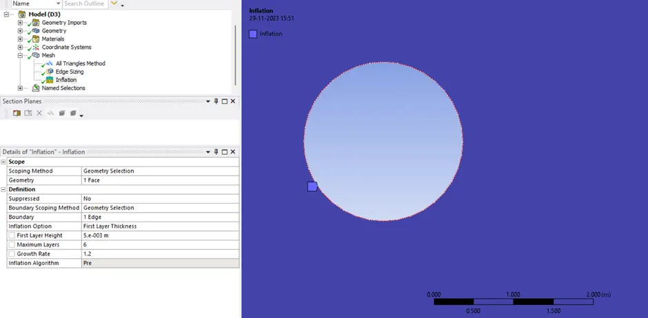
Change the element size
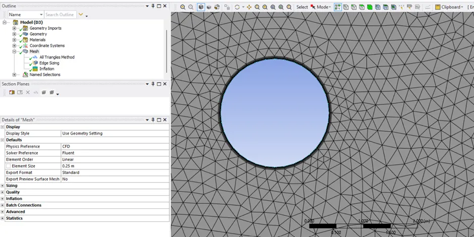
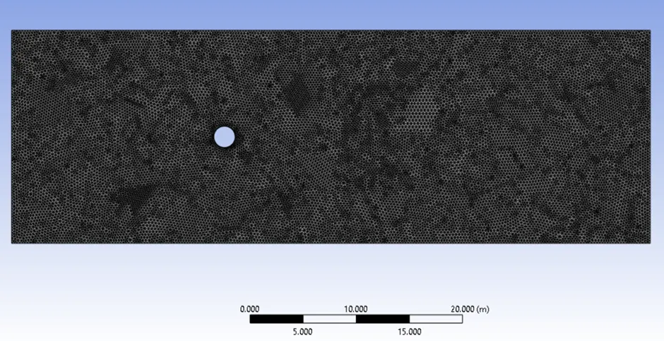
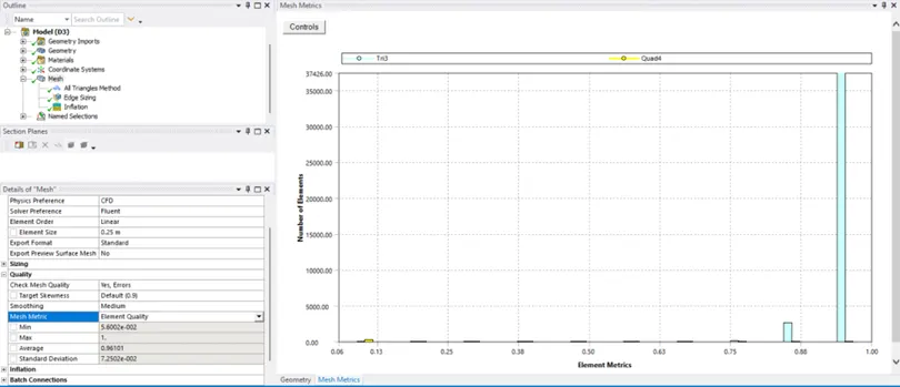
Quality of Mesh elements and elements metrics of the surface as shown in below picture.
Solver Setting
We have used customized fluid as working fluid which density is 1 kg/m3 and its viscosity will change according to the Reynolds number. Selected the pressure-based solver. We are using steady state solver and absolute velocity formation. We are interested in temperature study, so we choose the energy equation too. We have chosen the laminar viscous model because of Reynolds number is extremely small.
We have defined the boundary condition and added the appropriate values. Created the monitor point from the cylinder to 8m (4D).
Defined the plot of surface report of vortex average of velocity to the monitor point. Define the contour of velocity and pressure at all the components.
Analysis of all the cases
Case 1
1.1 Description of the case 1
Flow with the steady and Calculate the Strouhal Number for Re= 100
|
Description |
Values |
|
Flow type |
Steady state |
|
Turbulence \ Viscous model |
Laminar |
|
Inlet Velocity |
1 m/s |
|
Reynolds Number |
100 |
|
Working Fluid Density |
1 kg/m3 |
|
Working Fluid Viscosity |
0.02 kg/ms |
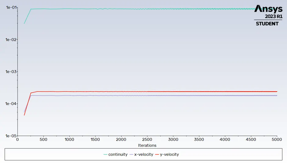
1.2 Line plot of Residual versus the iteration
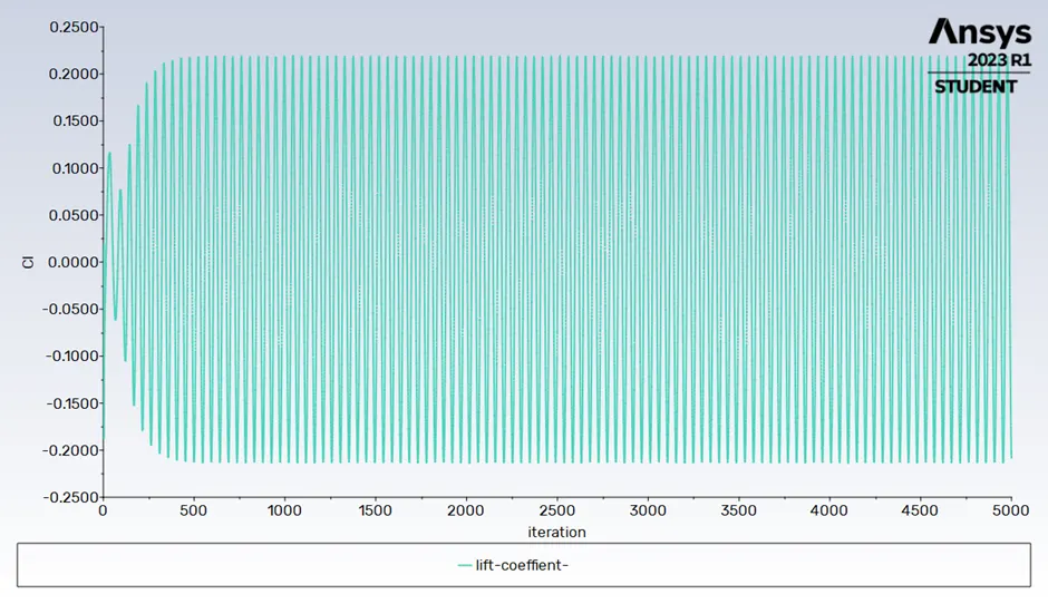
1.3 Line plot of lift coefficient versus the iteration
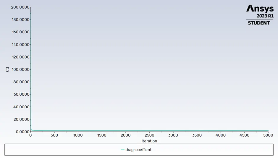
1.4 Line plot of Drag coefficient versus the iteration
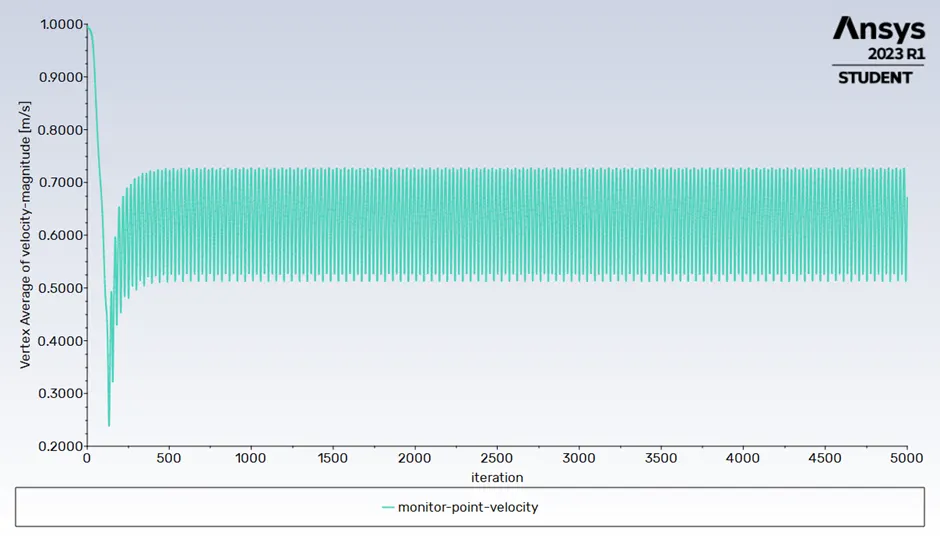
1.5 Velocity at monitor point versus the iteration
1.6 Pressure at monitor point versus the iteration
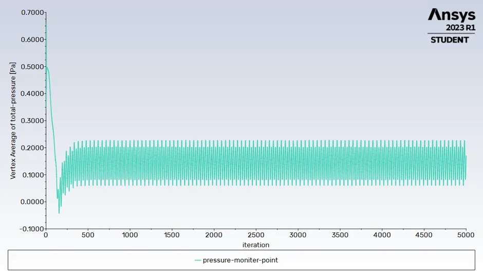
1.7 Result table
|
Description |
Values |
|
Pressure at Monitor Point |
0.1692 Pa |
|
Velocity at Monitor Point |
0.6741 m/s |
|
Lift Coefficient |
-0.2088 |
|
Drag Coefficient |
2.1604 |
|
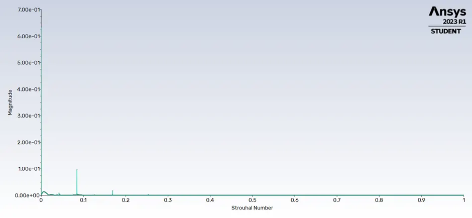
0.0843 |
1.8 Contour plot of velocity Magnitude
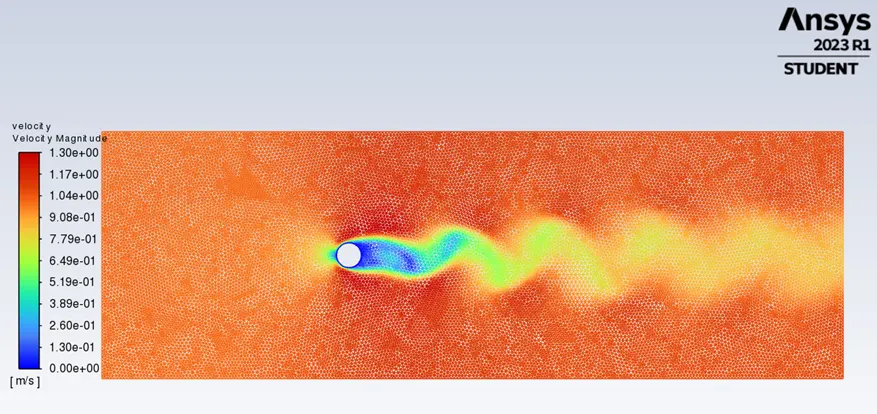
1.9 Contour Plot of total pressure
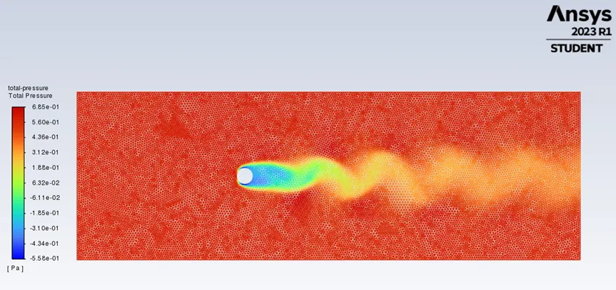
1.10 Contour Plot of Static Pressure
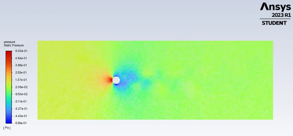
1.11 Magnitude vs Strouhal Number
Case 2
2.1 Description of the case 2
|
Description |
Values |
|
Flow type |
Unsteady state |
|
Turbulence \ Viscous model |
Laminar |
|
Inlet Velocity |
1 m/s |
|
Reynolds Number |
100 |
|
Working Fluid Density |
1 kg/m3 |
|
Working Fluid Viscosity |
0.02 kg/ms |
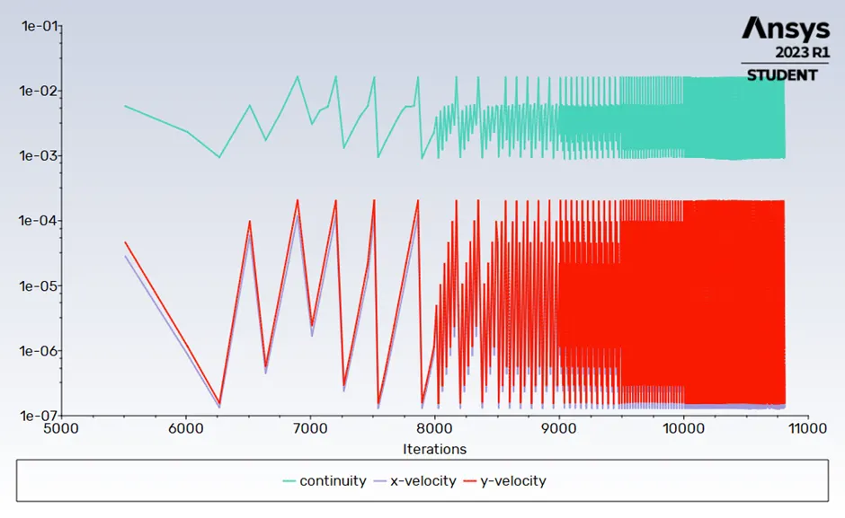
2.2 Line plot of Residual versus the iteration
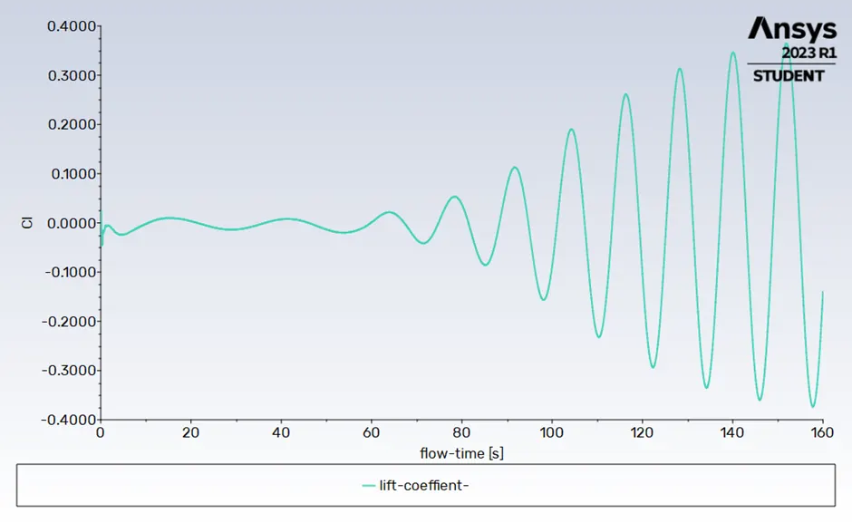
2.3 Line plot of lift coefficient versus the iteration
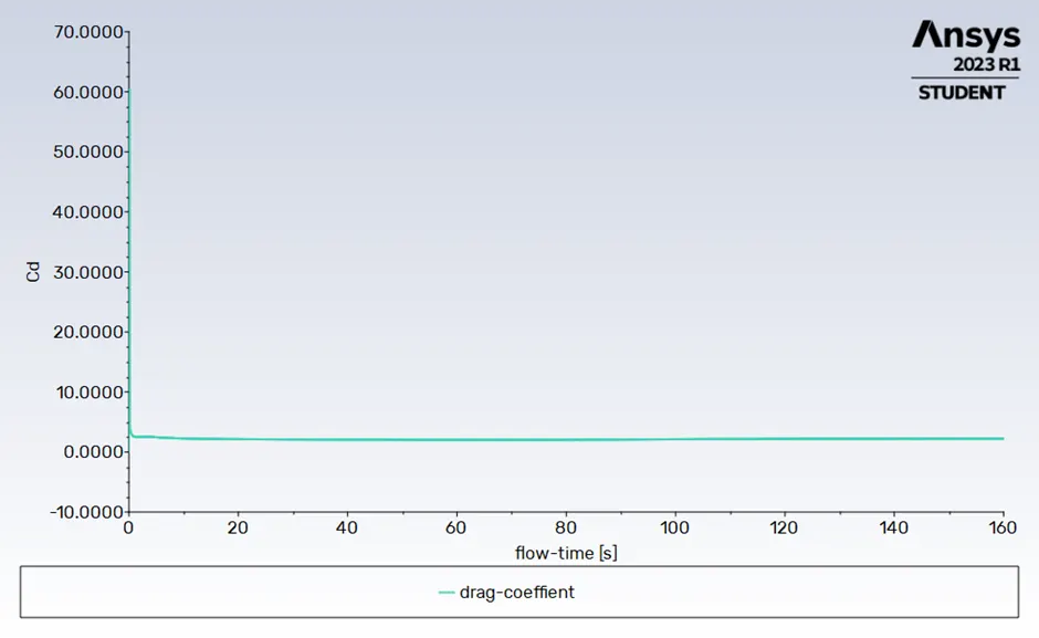
2.4 Line plot of Drag coefficient versus the iteration
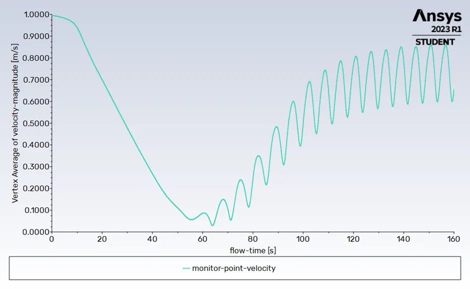
2.5 Velocity at monitor point versus the iteration
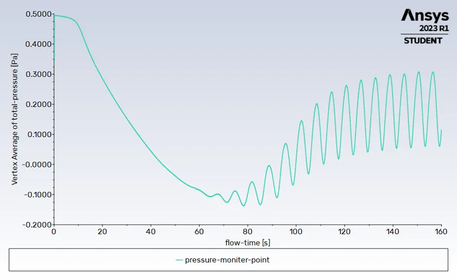
2.6 Pressure at monitor point versus the iteration
2.7 Result table
|
Description |
Values |
|
Pressure at Monitor Point |
0.1692 Pa |
|
Velocity at Monitor Point |
0.6532 m/s |
|
Lift Coefficient |
-0.13869 |
|
Drag Coefficient |
2.2301 |
|
Strouhal Number |
0.0309 |
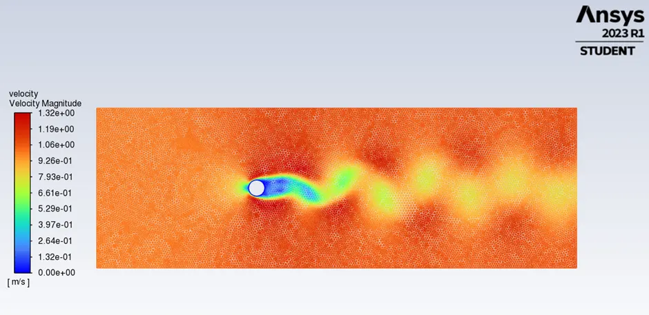
2.8 Contour plot of velocity Magnitude
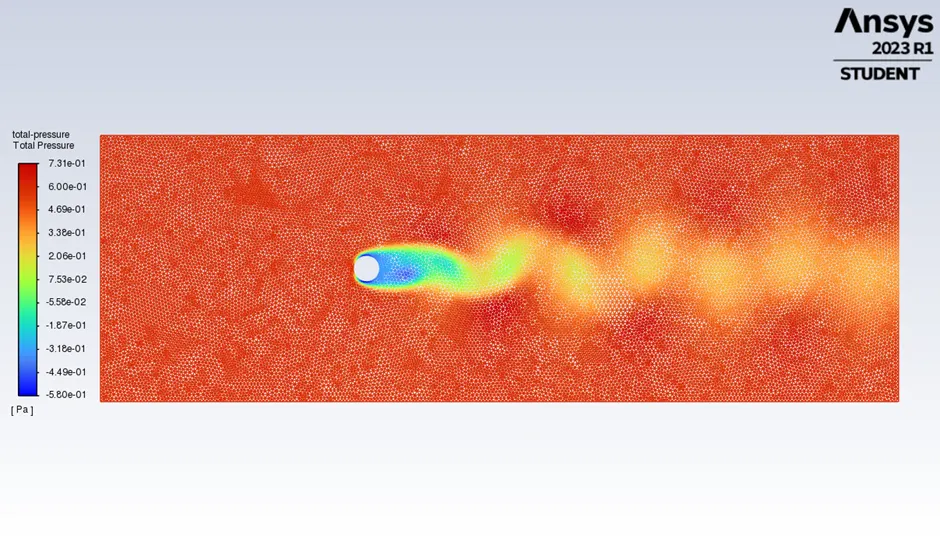
2.9 Contour Plot of total pressure
2.10 Contour Plot of Static pressure
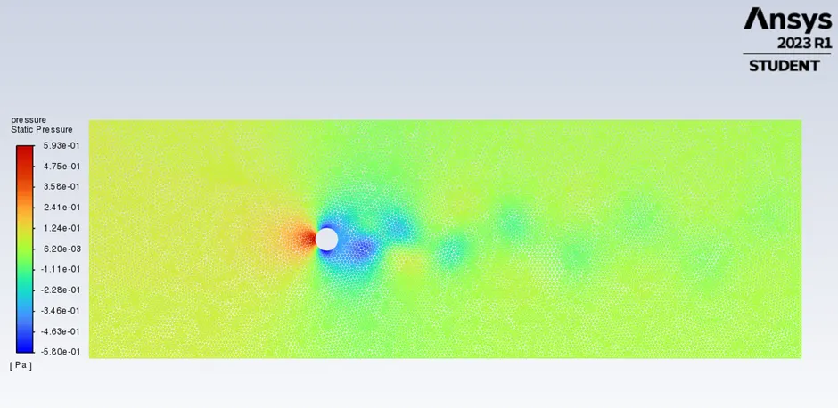
2.11 Magnitude vs Strouhal Number
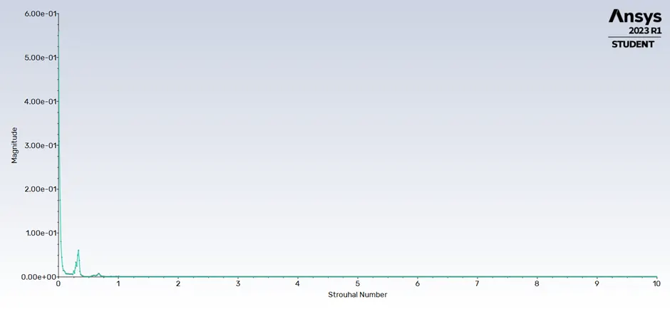
Case 3
Case 3
3.1 Description of the case 3
|
Description |
Values |
|
Flow type |
Steady state |
|
Turbulence \ Viscous model |
Laminar |
|
Inlet Velocity |
1 m/s |
|
Reynolds Number |
10 |
|
Working Fluid Density |
1 kg/m3 |
|
Working Fluid Viscosity |
0.2 kg/ms |
3.2 Line plot of Residual versus the iteration
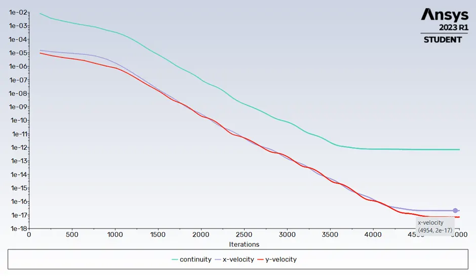
3.3 Line plot of lift coefficient versus the iteration
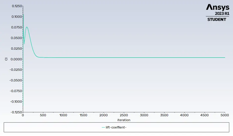
3.4 Line plot of Drag coefficient versus the iteration
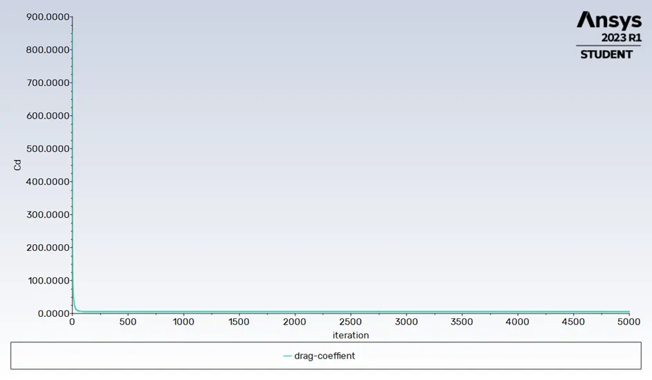
3.5 Velocity at monitor point versus the iteration
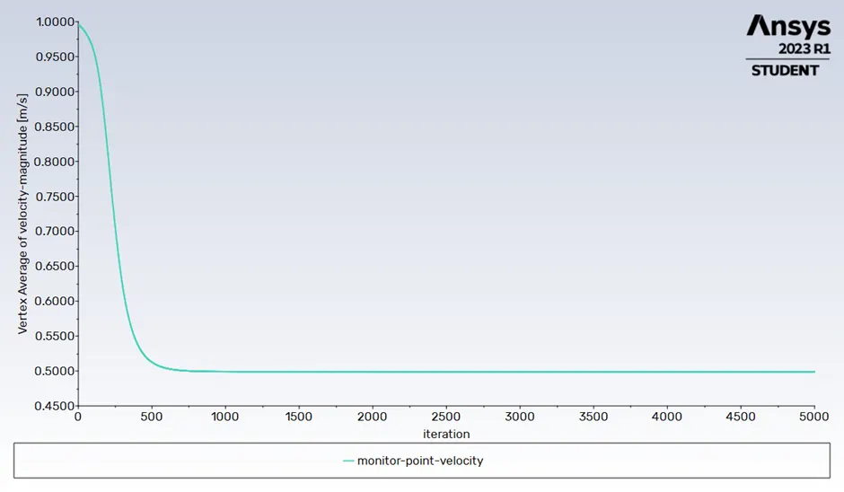
3.6 Pressure at monitor point versus the iteration
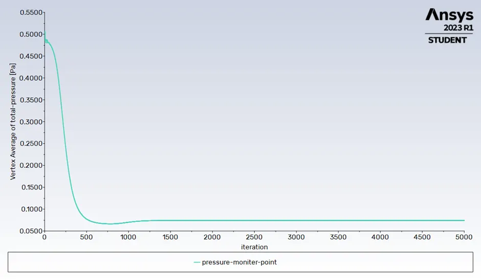
3.7 Result table
|
Description |
Values |
|
Pressure at Monitor Point |
0.0742 Pa |
|
Velocity at Monitor Point |
0.49896 m/s |
|
Lift Coefficient |
0.003555 |
|
Drag Coefficient |
3.3255 |
|
Strouhal Number |
- |
3.8 Contour plot of velocity Magnitude
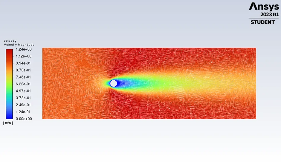
3.9 Contour Plot of total pressure
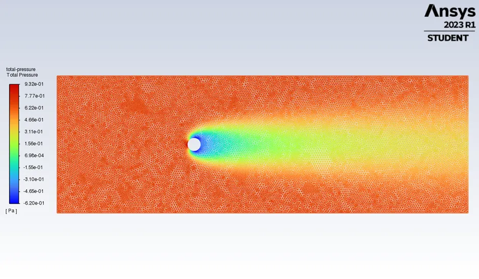
3.9 Contour Plot of total pressure
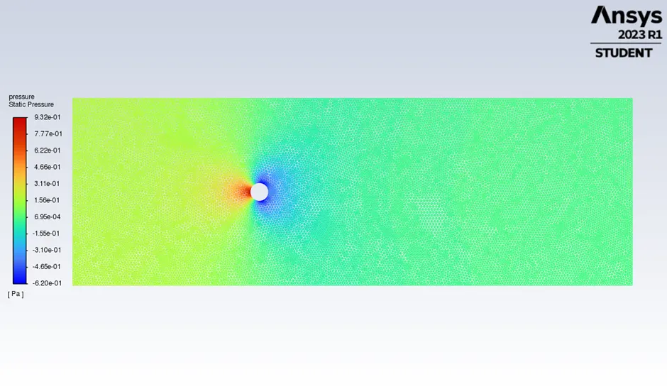
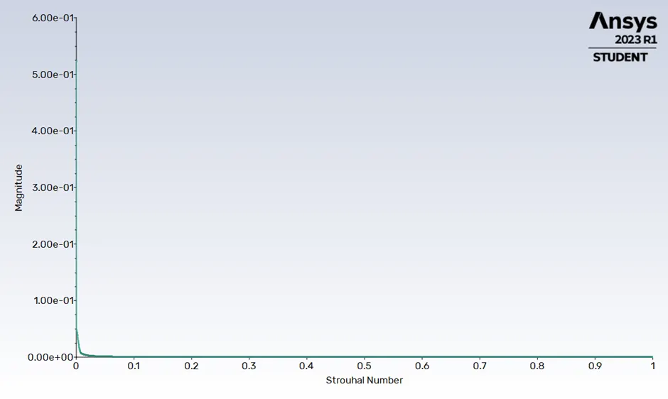
3.11 Magnitude vs Strouhal Number
Case 4
4.1 Description of the case 4
|
Description |
Values |
|
Flow type |
Steady state |
|
Turbulence \ Viscous model |
Laminar |
|
Inlet Velocity |
1 m/s |
|
Reynolds Number |
1000 |
|
Working Fluid Density |
1 kg/m3 |
|
Working Fluid Viscosity |
0.002 kg/ms |
4.2 Line plot of Residual versus the iteration
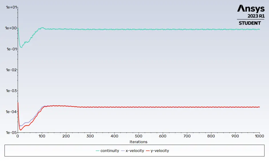
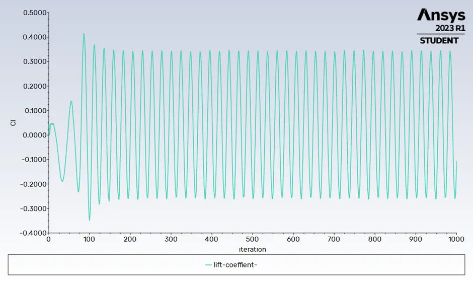
4.3 Line plot of lift coefficient versus the iteration
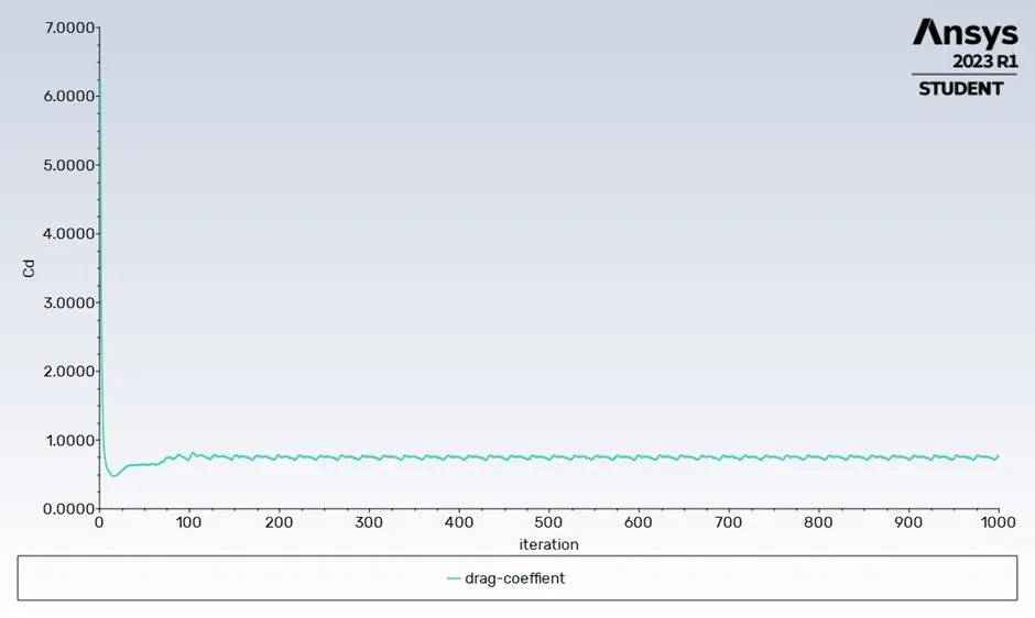
4.4 Line plot of Drag coefficient versus the iteration
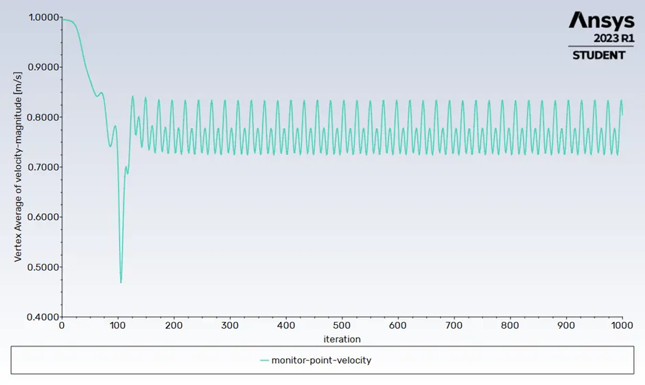
4.5 Velocity at monitor point versus the iteration
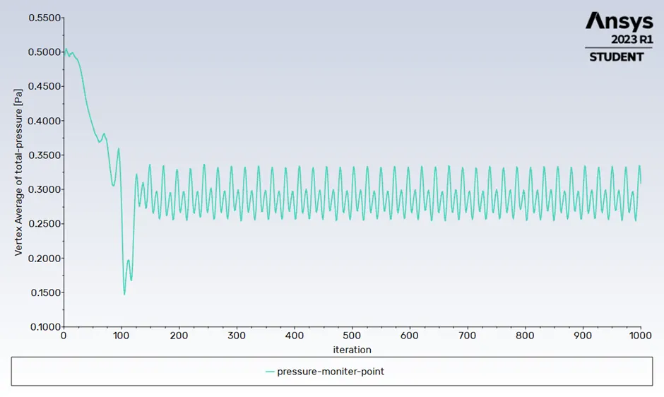
4.6 Pressure at monitor point versus the iteration
4.7 Result table
|
Description |
Values |
|
Pressure at Monitor Point |
0.3090 Pa |
|
Velocity at Monitor Point |
0.80398 m/s |
|
Lift Coefficient |
-0.1065 |
|
Drag Coefficient |
0.7663 |
|
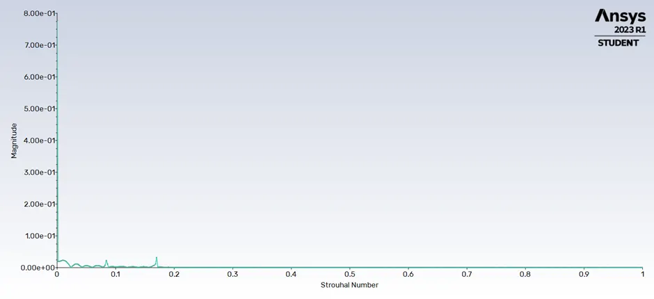
Strouhal Number |
0.168 |
4.8 Contour plot of velocity Magnitude
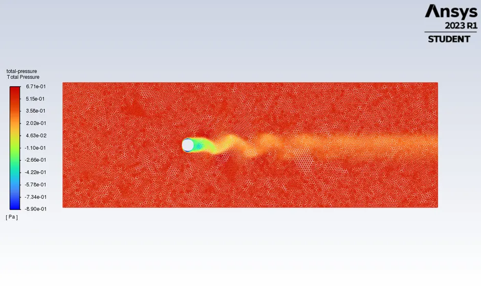
4.9 Contour Plot of total pressure
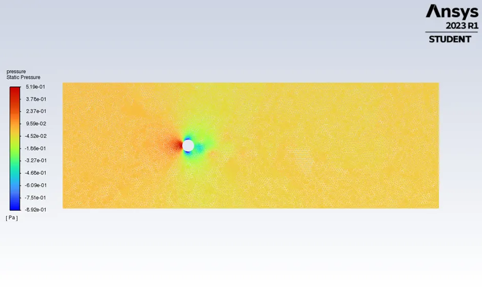
4.10 Contour Plot of Static pressure
4.11 Magnitude vs Strouhal Number
Conclusion
1.Strauhal number
Strauhal number calculated for steady state with Reynolds number 100 is .0843
Strauhal number calculated for Unsteady state with Reynolds number 100 is 0.031
2.coefficient of drag and lift
|
Reynolds Number |
Coefficient of Drag |
Coefficient of Lift |
|
10 |
3.3255 |
0.0036 |
|
100 Steady |
2.1604 |
0.02088 |
|
100 Unsteady/Transient |
2.2301 |
0.03388 |
|
1000 |
0.7663 |
0.1065 |
|
10000 |
1.5279 |
0.2499 |
|
100000 |
0.8687 |
0.5325 |
By comparing result table of all the cases, increase in the Reynolds decreases the coefficient of drag so that Reynolds number inversely proportional to coefficient of drag.