Challenge

Week 7 - Simulation of a 1D Supersonic nozzle flow simulation using Macormack Method

RRanjith Kumarb15 Jul 2024

NOTE: I could not find the insert code and inert equation option here. so pasted the pictures and program as it is.

Aim

1. To solve the 1D supersonic nozzle flow equation

2. To plot Steady-state distribution of primitive variables inside the nozzle

3. To plot the Time-wise variation of the primitive variables

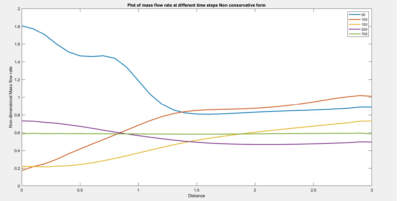
4. To plot the Variation of Mass flow rate distribution inside the nozzle at different time steps during the time-marching process

5. To Comparison of Normalized mass flow rate distributions of conservative and non-conservative forms

6. To Perform a grid independence test on the solution and explain all your findings.

Introduction:

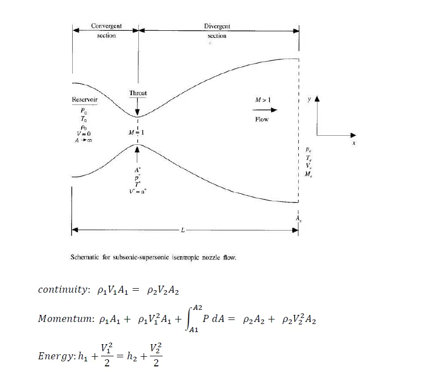
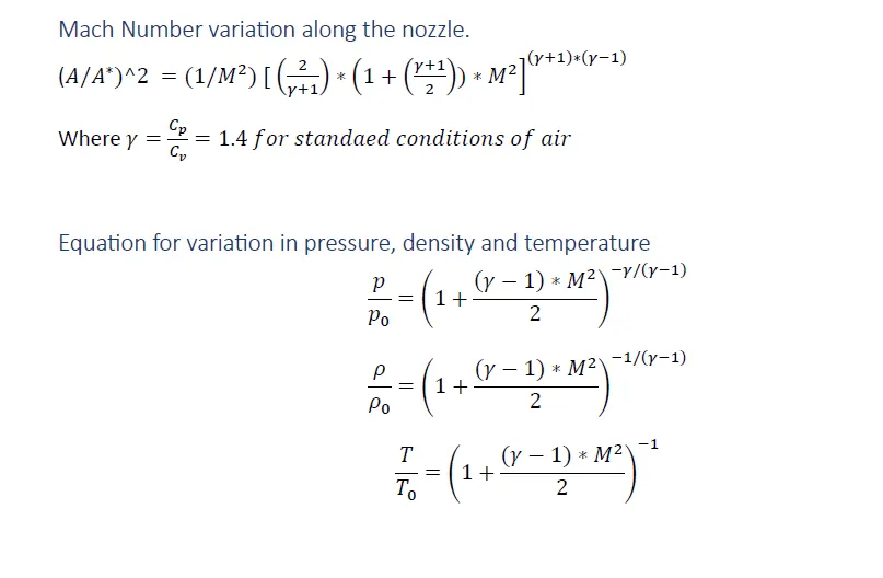
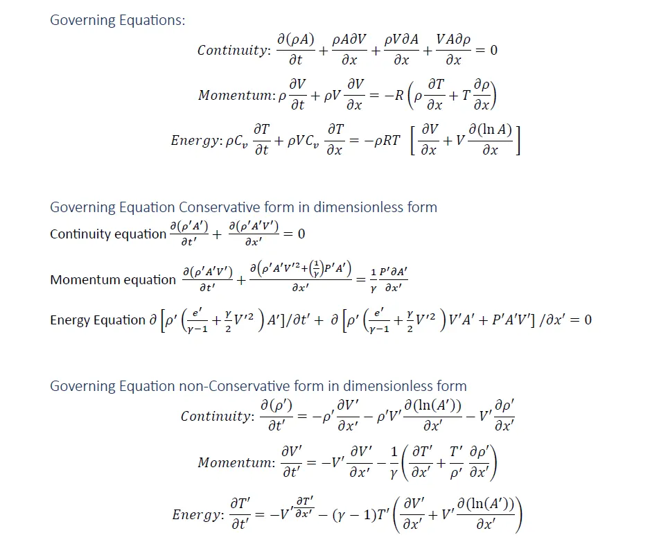
We consider the steady, isentropic flow through a convergent-divergent nozzle. The flow at the inlet to the nozzle comes from a reservoir where pressure and temperatures are at stagnation. Also, it is assumed that the cross-sectional area of the nozzle is very large so that the velocity is almost V ~ 0. The flow expands adiabatically to supersonic speeds at the nozzle exit. the flow is locally subsonic in the convergent section (M < 1), sonic at the throat section (M = 1) and supersonic at the divergent section (M> 1). We assume that at a given section, where the cross-sectional area is A, the flow properties are uniform across the section. Hence although the area of the nozzle changes as the function of distance along the nozzle x, and therefore in reality the flow field is two-dimensional (the flow varies in two dimensional xy space), we make the assumption that the flow properties vary only with x, such flow is defined as Quasi one dimensional flow.

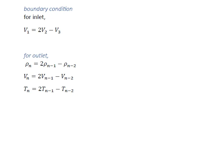
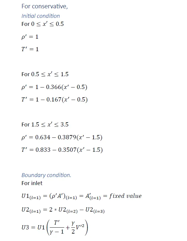
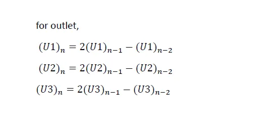
Code

Main Program

clear all

close all

clc

n=input('enter number of grid points=');

nt=input('enter number of time steps=');

C=input('enter courant number/CFL number=');

[rho,v,T,M,P,mfr,P_t,rho_t,T_t,M_t]=conservative(n,nt,C);

rho_c=rho;

v_c=v;

T_c=T;

M_c=M;

P_c=P;

mfr_c=mfr;

P_tc=P_t;

rho_tc=rho_t;

T_tc=T_t;

M_tc=M_t;

[rho,v,T,M,P,mfr,P_t,rho_t,T_t,M_t]=non_conservative(n,nt,C);

figure(4)

x=linspace(0,3,n);

plot(x,mfr_c)

hold on

plot(x,mfr)

line([0 3],[0.579 0.579],'linewidth',1,'color','g');

title_text=sprintf( 'Mass flow rate Vs Distance for %d Grid points',n);

title(title_text);

legend ('Conservative','Non-Conservative', 'Analytical Solution');

xlabel('x/L, nondimensional distance');

ylabel('Mass flow rate m');

For Non conservative,

function [rho,v,T,M,P,mfr,P_t,rho_t,T_t,M_t]=non_conservative(n,nt,C)

%non conservative form

%Inputs

x=linspace(0,3,n);

dx=x(2)-x(1);

A=1+(2.2*((x-1.5).^2)); % Area

%initial Conditions

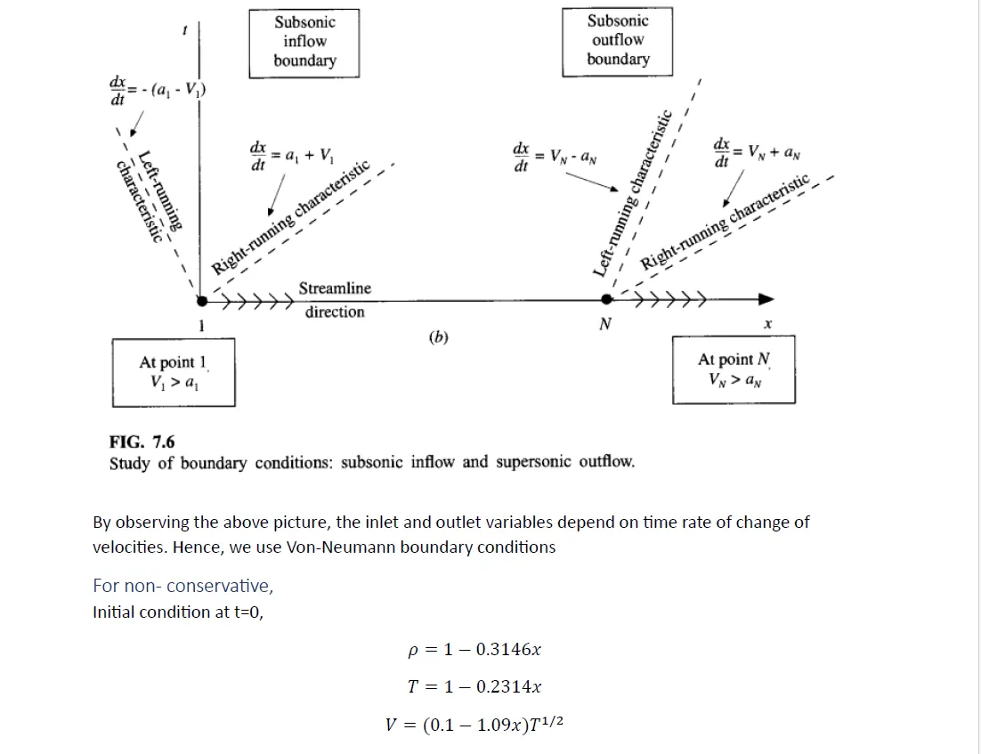
rho=1-(0.3146*x); % Density non Dimensional qty.

T=1-(0.2314*x); % Temperature non Dimensional qty.

v=(0.1+(1.09*x)).*(T.^0.5); % velocity non Dimensional qty.

%a0 is the speed of sound in resrvoir=sqrt(gamma*R*T0)

dt=min((C.*dx)./(sqrt(T)+v)); %dt=0.001;magnitude of time step

gamma=1.4;

%outer time loop

for k=1:nt

rho_old=rho;

v_old=v;

T_old=T;

%predictor step

for j=2:n-1

dvdx=((v(j+1)-v(j))/dx);

drhodx=((rho(j+1)-rho(j))/dx);

dTdx=((T(j+1)-T(j))/dx);

dlnAdx=((log(A(j+1))-log(A(j)))/dx);

% continuinity equation

drhodt_p(j)=-(rho(j)*dvdx)-(rho(j)*v(j)*dlnAdx)-(v(j)*drhodx);

% Momentum equation

dvdt_p(j)=-(v(j)*dvdx)-((1/gamma)*(dTdx+((T(j)/rho(j)))*(drhodx)));

% Energy equation

dTdt_p(j)=-(v(j)*dTdx)-(gamma-1)*(T(j)*(dvdx+(v(j)*dlnAdx)));

%solution update

rho(j)=rho(j)+(drhodt_p(j)*dt);

v(j)=v(j)+(dvdt_p(j)*dt);

T(j)=T(j)+(dTdt_p(j)*dt);

end

%corrector step

for j=2:n-1

dvdx=((v(j)-v(j-1))/dx);

drhodx=((rho(j)-rho(j-1))/dx);

dTdx=((T(j)-T(j-1))/dx);

dlnAdx=((log(A(j))-log(A(j-1)))/dx);

% continuinity equation

drhodt_c(j)=-(rho(j)*dvdx)-(rho(j)*v(j)*dlnAdx)-(v(j)*drhodx);

% Momentum equation

dvdt_c(j)=-(v(j)*dvdx)-((1/gamma)*(dTdx+((T(j)/rho(j)))*(drhodx)));

% Energy equation

dTdt_c(j)=-(v(j)*dTdx)-(gamma-1)*(T(j)*(dvdx+(v(j)*dlnAdx)));

end

% average time derivative

drhodt=0.5*(drhodt_p+drhodt_c);

dvdt=0.5*(dvdt_p+dvdt_c);

dTdt=0.5*(dTdt_p+dTdt_c);

%final solution

for i=2:n-1

rho(i)=rho_old(i)+(drhodt(i)*dt);

v(i)=v_old(i)+(dvdt(i)*dt);

T(i)=T_old(i)+(dTdt(i)*dt);

end

%apply for boundary condition

%inlet

v(1)=2*v(2)-v(3);

%outlet

rho(n)=2*rho(n-1)-rho(n-2);

v(n)=2*v(n-1)-v(n-2);

T(n)=2*T(n-1)-T(n-2);

%mach Number

M=v./sqrt(T);

%pressure

P=rho.*T;

%mass flow rate

mfr=rho.*v.*A;

% Throat datas

throat= find(A==1);

rho_t(k)=rho(throat);

T_t(k)=T(throat);

v_t(k)=v(throat);

P_t(k)=P(throat);

M_t(k)=M(throat);

%Steady-state distribution of primitive variables inside the nozzle

figure(11)

subplot(5,1,1)

plot(x,v)

title(sprintf('Non conservative \n velocity vs Distance Time step= %d',k))

xlabel('Length of nozzel')

ylabel('Velocity')

subplot(5,1,2)

plot(x,rho)

title(sprintf('density vs Distance Time step= %d',k))

xlabel('Length of nozzel')

ylabel('Density')

subplot(5,1,3)

plot(x,T)

title(sprintf('Temperature vs Distance, Time step= %d',k))

xlabel('Length of nozzel')

ylabel('temperature')

subplot(5,1,4)

plot(x,M)

title(sprintf('Mach Number vs Distance, Time step= %d',k))

xlabel('Length of nozzel')

ylabel('Mach Number')

subplot(5,1,5)

plot(x,P)

title(sprintf('Pressure vs Distance, Time step= %d',k))

xlabel('Length of nozzel')

ylabel('Pressure')

%if else condition to plot the variation of non dimensional mass flow rate at specific time steps and plot the same

figure(13)

if k == 50

%plotting of mass flow rate at time step 50

plot(x,mfr,'Linewidth', 2)

hold on

elseif k == 100

%plotting of mass flow rate at time step 100

plot (x,mfr,'Linewidth', 2)

elseif k==150

%plotting of mass flow rate at time step 150

plot(x,mfr,'Linewidth', 2)

elseif k==200

%plotting of mass flow rate at time step 200

plot (x,mfr,'Linewidth', 2)

elseif k==700

%plotting of mass flow rate at time step 700

plot (x,mfr,'Linewidth', 2)

title ('Plot of mass flow rate at different time steps Non conservative form')

xlabel('Distance')

ylabel('Non-dimensional Mass flow rate')

legend ('50','100','150','200','700')

end

%Time-wise variation of the primitive variables

nt=1:1400;

figure(12)

subplot(5,1,1)

plot(nt,v_t)

title(sprintf('Non conservative \n velocity vs Timestep, Gridpoints= %d',n))

xlabel('Time step')

ylabel('Velocity')

subplot(5,1,2)

plot(nt,rho_t)

title(sprintf('density vs Timestep, Gridpoints= %d',n))

xlabel('Time step')

ylabel('Density')

subplot(5,1,3)

plot(nt,T_t)

title(sprintf('Temperature vs Timestep, Gridpoints= %d',n))

xlabel('Time step')

ylabel('temperature')

subplot(5,1,4)

plot(nt,M_t)

title(sprintf('Mach Number vs Timestep, Gridpoints= %d',n))

xlabel('Time step')

ylabel('Mach Number')

subplot(5,1,5)

plot(nt,P_t)

title(sprintf('Pressure vs Timestep, Gridpoints= %d',n))

xlabel('Time step')

ylabel('Pressure')

For conservative,

function[rho,v,T,M,P,mfr,P_t,rho_t,T_t,M_t]=conservative(n,nt,C)

%Conservation form

%Inputs

x=linspace(0,3,n);

dx=x(2)-x(1);

%initial Conditions

for i=1:length(x)

if (x(i)<=0.5)

rho(i)=1;

T(i)=1;

end

for i=1:length(x)

if (x(i)>0.5) && (x(i)<=1.5)

rho(i)=1-(0.366*(x(i)-0.5)); % Density non Dimensional qty.

T(i)=1-(0.167*(x(i)-0.5));

end

for i=1:length(x)

if (x(i)>1.5) && (x(i)<=3.5)

rho(i)=0.634-(0.3879*(x(i)-1.5));

T(i)=0.833-(0.3507*(x(i)-1.5));

end

A=1+(2.2*((x-1.5).^2)); % Area

v=0.59./(rho.*A); %velocity

%a0 is the speed of sound in resrvoir=sqrt(gamma*R*T0)

dt=min((C.*dx)./(sqrt(T)+v)); %dt=0.001;magnitude of time step

gamma=1.4; %cp/Cv

%solution vector equations

U1=rho.*A;

U2=rho.*A.*v;

U3=rho.*((T./(gamma-1))+(gamma/2).*v.^2).*A;

for k=1:nt

U1_old=U1;

U2_old=U2;

U3_old=U3;

for j=2:n-1

%flux vector equations, Initialization of flux

F1=U2;

F2=((U2.^2)./U1)+((gamma-1)/gamma)*(U3-(gamma/2)*(((U2).^2)./U1));

F3=(((gamma)*(U2.*U3))./U1)-(((gamma*(gamma-1))/2)*((U2.^3)./U1.^2));

%predictor step

J2(j)=(1/gamma)*rho(j)*T(j)*((A(j+1)-A(j))/dx);

dU1dt_p(j)=-((F1(j+1)-F1(j))/dx);

dU2dt_p(j)=-((F2(j+1)-F2(j))/dx)+J2(j);

dU3dt_p(j)=-((F3(j+1)-F3(j))/dx);

% solution update

U1(j)=U1(j)+(dU1dt_p(j)*dt);

U2(j)=U2(j)+(dU2dt_p(j)*dt);

U3(j)=U3(j)+(dU3dt_p(j)*dt);

end

rho=(U1./A);

v=(U2./U1);

T= (gamma-1)*((U3./U1)-(gamma/2)*(v).^2);

p=rho.*T; %pressure

%Updating the flux vector F1,F2,F3

F1=U2;

F2=((U2.^2)./U1)+((gamma-1)/gamma)*(U3-(gamma/2)*(((U2).^2)./U1));

F3=(((gamma)*(U2.*U3))./U1)-(((gamma*(gamma-1))/2)*((U2.^3)./U1.^2));

%corrector step

for j=2:n-1

J2(j)=(1/gamma)*rho(j)*T(j)*((A(j)-A(j-1))/dx);

dU1dt_c(j)=-((F1(j)-F1(j-1))/dx);

dU2dt_c(j)=-((F2(j)-F2(j-1))/dx)+J2(j);

dU3dt_c(j)=-((F3(j)-F3(j-1))/dx);

end

% average time derivative

dU1dt= 0.5*(dU1dt_p+dU1dt_c);

dU2dt=0.5*(dU2dt_p+dU2dt_c);

dU3dt=0.5*(dU3dt_p+dU3dt_c);

%final solution

for i=2:n-1

U1(i)=U1_old(i)+(dU1dt(i)*dt);

U2(i)=U2_old(i)+(dU2dt(i)*dt);

U3(i)=U3_old(i)+(dU3dt(i)*dt);

end

rho=(U1./A);

v=(U2./U1);

T= (gamma-1)*((U3./U1)-(gamma/2)*(v).^2);

p=rho.*T; %pressure

%apply for boundary condition

%inlet

U1(1)=A(1);

U2(1)=2*U2(2)-U2(3);

U3=U1.*((T./(gamma-1))+(0.5*gamma.*(v.^2)));

%outlet

U1(n)=2*U1(n-1)-U1(n-2);

U2(n)=2*U2(n-1)-U2(n-2);

U3(n)=2*U3(n-1)-U3(n-2);

%mach Number

M=v./sqrt(T);

%pressure

P=rho.*T;

%mass flow rate

mfr=rho.*v.*A;

% Throat datas

throat= find(A==1);

rho_t(k)=rho(throat);

T_t(k)=T(throat);

v_t(k)=v(throat);

P_t(k)=P(throat);

M_t(k)=M(throat);

%Steady-state distribution of primitive variables inside the nozzle

figure(1)

subplot(5,1,1)

plot(x,v)

title(sprintf('conservative \n velocity vs Distance Time step= %d',k))

xlabel('Length of nozzel')

ylabel('Velocity')

subplot(5,1,2)

plot(x,rho)

title(sprintf('density vs Distance Time step= %d',k))

xlabel('Length of nozzel')

ylabel('Density')

subplot(5,1,3)

plot(x,T)

title(sprintf('Temperature vs Distance, Time step= %d',k))

xlabel('Length of nozzel')

ylabel('temperature')

subplot(5,1,4)

plot(x,M)

title(sprintf('Mach Number vs Distance, Time step= %d',k))

xlabel('Length of nozzel')

ylabel('Mach Number')

subplot(5,1,5)

plot(x,P)

title(sprintf('Pressure vs Distance, Time step= %d',k))

xlabel('Length of nozzel')

ylabel('Pressure')

%if else condition to plot the variation of non dimensional mass flow rate at specific time steps and plot the same

figure(3)

if k == 50

%plotting of mass flow rate at time step 50

plot(x,mfr,'Linewidth', 2)

hold on

elseif k == 100

%plotting of mass flow rate at time step 100

plot (x,mfr,'Linewidth', 2)

elseif k==150

%plotting of mass flow rate at time step 150

plot(x,mfr,'Linewidth', 2)

elseif k==200

%plotting of mass flow rate at time step 200

plot (x,mfr,'Linewidth', 2)

elseif k==700

%plotting of mass flow rate at time step 700

plot (x,mfr,'Linewidth', 2)

title ('Plot of mass flow rate at different time steps conservative form')

xlabel('Distance')

ylabel('Non-dimensional Mass flow rate')

legend ('50','100','150','200','700')

end

%Time-wise variation of the primitive variables

nt=1:1400;

figure(2)

subplot(5,1,1)

plot(nt,v_t)

title(sprintf('conservative \n velocity vs Timestep, Gridpoints= %d',n))

xlabel('Time step')

ylabel('Velocity')

subplot(5,1,2)

plot(nt,rho_t)

title(sprintf('density vs Timestep, Gridpoints= %d',n))

xlabel('Time step')

ylabel('Density')

subplot(5,1,3)

plot(nt,T_t)

title(sprintf('Temperature vs Timestep, Gridpoints= %d',n))

xlabel('Time step')

ylabel('temperature')

subplot(5,1,4)

plot(nt,M_t)

title(sprintf('Mach Number vs Timestep, Gridpoints= %d',n))

xlabel('Time step')

ylabel('Mach Number')

subplot(5,1,5)

plot(nt,P_t)

title(sprintf('Pressure vs Timestep, Gridpoints= %d',n))

xlabel('Time step')

ylabel('Pressure')

end

Results

Non-Conservative

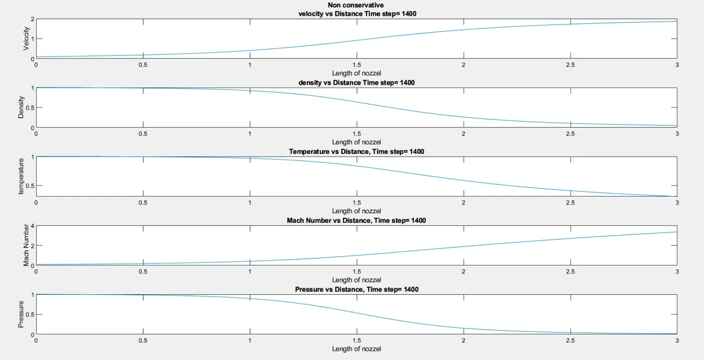
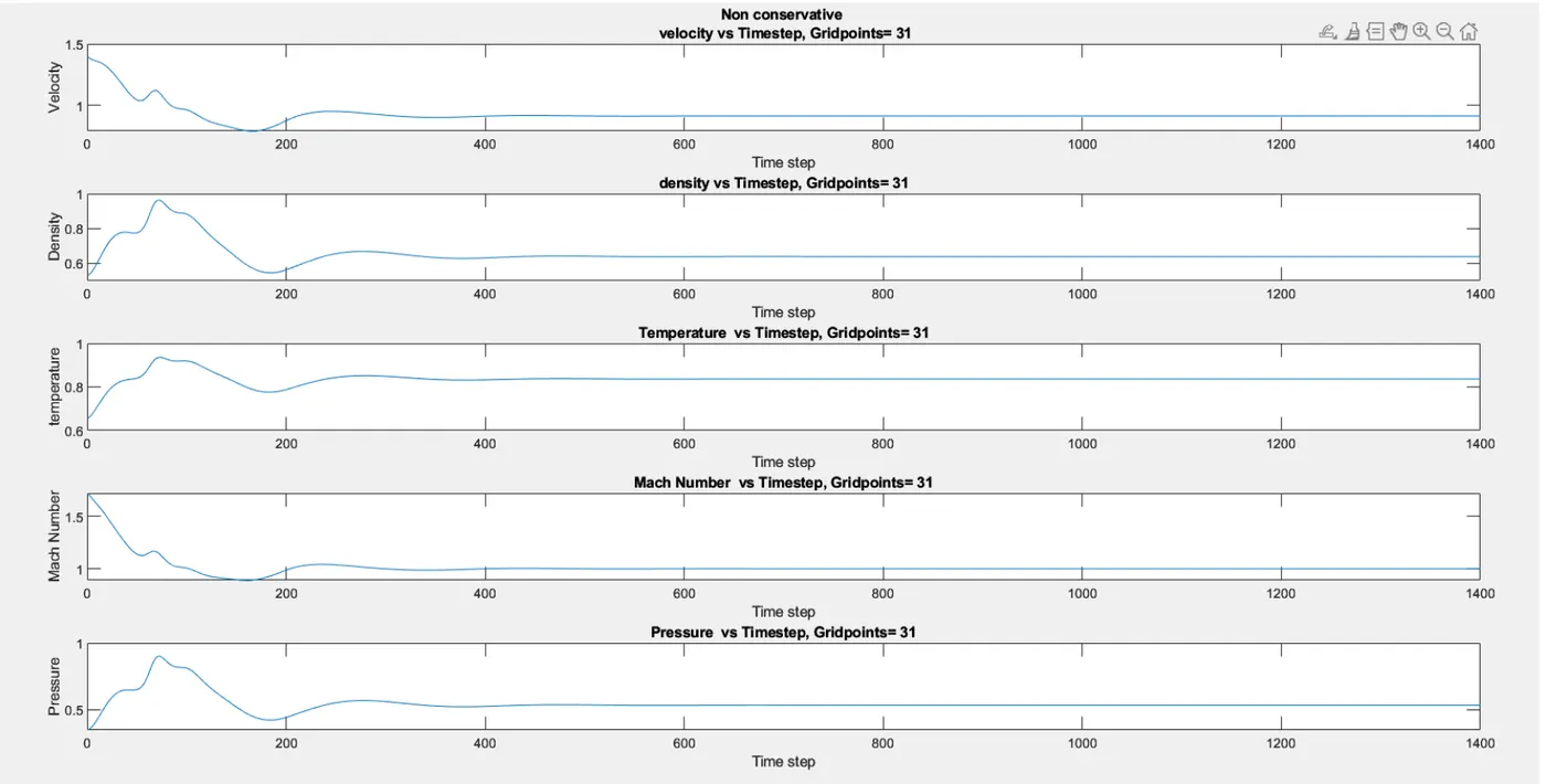
At throat

Conservative

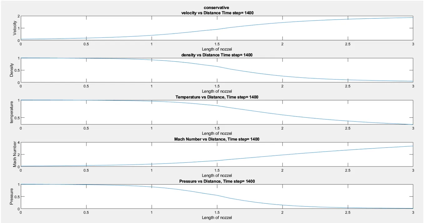
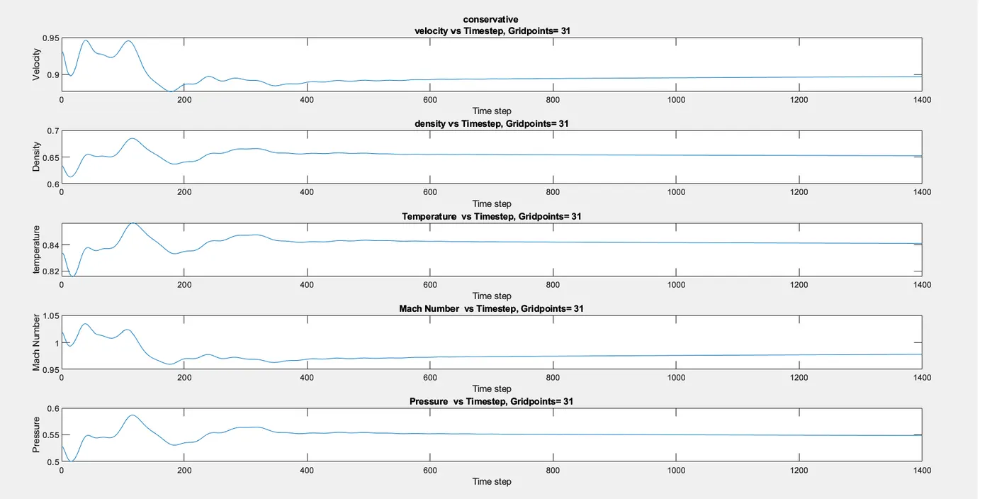
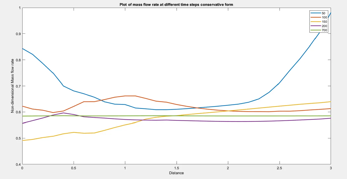
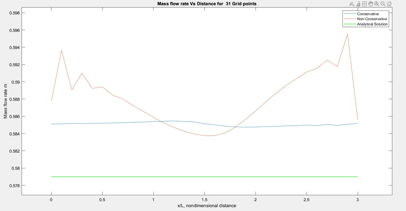
As per above plots,

1. Velocity and Mach number increase with the length of the nozzle. Density, temperature and pressure decreases with length of the nozzle.

2. If we observe throat values with respect to the time steps. Initial time steps values not stable after some steps it will become stable

3. By observing the mass flow rate plot, conservative form is more stable than non-conservative form. Conservative form is closer to analytical solution.

Grid Independent test

Flow Variables at Throat	Analytical solution	Conservative		Non- conservative
Flow Variables at Throat	Analytical solution	n=61	n=31	n=61	n=31
Density	0.634	0.6390	0.6524	0.6377	0.6387
Temperature	0.8733	0.8357	0.8411	0.8355	0.8365
Pressure	0.528	0.5340	0.5487	0.5327	0.5342
Mach Number	1	0.9978	0.9797	0.9998	0.9994

From the above results we can see that for a grid-size of 30 points the Non-Conservative form gives a more accurate result compared to the Conservative form. However when we change the grid-size to 60 points the values of the flow quantities are quite close when calculated by either of the methods

CONCLUSION:

1. Better mass flow rate distribution is done in conservation form.

2. Non conservation form easy to write the code, where conservative form is complex because we calculate the primitive variable through flux variable.

3. Non conservative form provides less error compare to conservative form so accuracy is better in non-conservative form

4. In non-conservation form behaviour of the residuals are good as compare to conservation form. The residuals decays faster in non-conservation form when compared to conservation form

5. The primitive variables converge to a numerical steady-state faster when using the non-conservation form

Week 7 - Simulation of a 1D Supersonic nozzle flow simulation using Macormack Method

Aim

2. To plot Steady-state distribution of primitive variables inside the nozzle

3. To plot the Time-wise variation of the primitive variables

4. To plot the Variation of Mass flow rate distribution inside the nozzle at different time steps during the time-marching process

5. To Comparison of Normalized mass flow rate distributions of conservative and non-conservative forms

Introduction:

Code

Main Program

For Non conservative,

For conservative,

Results

CONCLUSION:

Ship work like this
in your own course.

Talk to a career counsellor

Aim

2. To plot Steady-state distribution of primitive variables inside the nozzle

3. To plot the Time-wise variation of the primitive variables

4. To plot the Variation of Mass flow rate distribution inside the nozzle at different time steps during the time-marching process

5. To Comparison of Normalized mass flow rate distributions of conservative and non-conservative forms

Introduction:

Code

Main Program

For Non conservative,

For conservative,

Results

CONCLUSION:

Ship work like thisin your own course.

Talk to a career counsellor

Ship work like this
in your own course.