Aim:

· To give a brief description of why and where a CHT analysis is used.

· To maintain the y+ value according to the turbulence model and justify the results.

· To calculate the wall/surface heat transfer coefficient on the internal solid surface & show the velocity & temperature contours in appropriate areas.

· To get answer for how would you verify if the HTC predictions from the simulations are right? On what factors does the accuracy of the prediction depend on?

Introduction:

CHT Analysis and Its Importance

Conjugate heat transfer is a type of heat transfer analysis between solids and fluid. This type of heat transfer includes both convection (between fluids) and conductive (between solids) heat transfer, as well as both forced and natural convection. Common applications and use cases of this thermal simulation type include electronics cooling, heat exchangers, industrial machinery.

In solids, heat transfer typically occurs through conduction, while in fluids, it happens through convection. Conjugate heat transfer combines these two mechanisms to provide a comprehensive understanding of the thermal interactions between solids and fluids. For example, in a heat sink, heat is conducted through the solid material and then transferred to the surrounding fluid by convection.

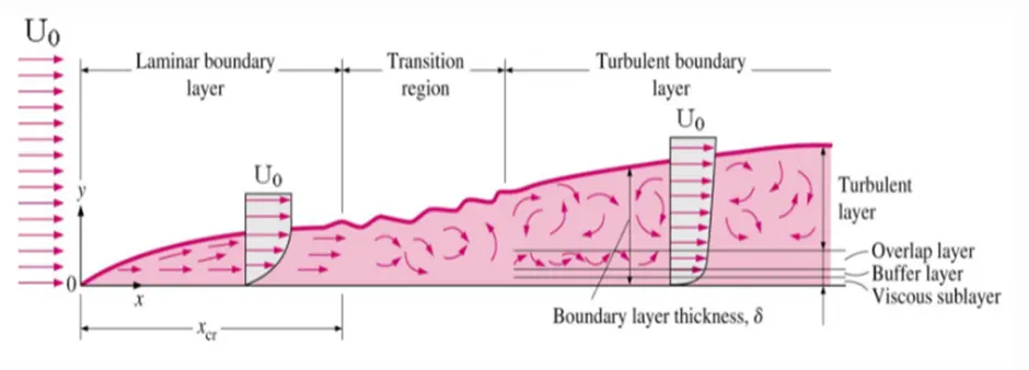
Growth of the Boundary layer over the plate.

Y+ Value

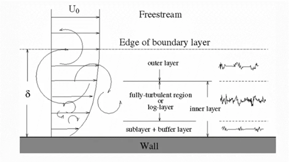
Here y plus values are selected in accordance with the turbulence model we choose to solve the problem with. So particular. turbulence model have its own range of y plus values to get more accurate results

Y+> 500 for the outer layer

30<Y+<500 for log low region (High Reynolds number formulation hence K-epsilon is used)

5<Y+<30 for the buffer layer

Y+<5 for viscous sublayer (low Reynolds number formulation hence K-w or SST is used)

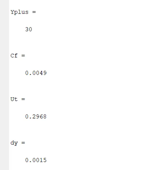
Y+ calculation by Matlab

clear all

close all

clc

Re = 67934; %Reynolds number

rho = 1.225; %density of the fluid

U = 6; %velocity

Yplus = 30

Mu = 1.7965e-5; %dynamic viscosity

Cf = 0.079*Re^(-0.25) %for internal flow, skin friction factor which is function of Reynolds number.

Tw = 0.5*(Cf*rho*U^2); % wall shear stress

Ut = (Tw/rho)^0.5 % frictional velocity

dy = (Yplus*Mu)/(rho*Ut) %first cell height

result

Matlab Calculation for Heat transfer coefficient

close all

clear all

clc

%input

rho= 1.225; % density kg/m^3

mu= 1.796e-5; %dynamic viscosity

U = 6; %velocity in m/s

D= 0.166; %Pipe diameter in m

Pr=0.746; %Prandtl number

L=D; %Characteristic length

k=0.0242; %thermal conductivity of the fluid

%Reynolds Number

Re=(rho*U*D)/mu

%Nusselt Number

Nu=0.023*(Re^0.8)*(Pr^0.4)

%heat transfer coefficient in W/m^2 K

h=Nu*(k/L)

Result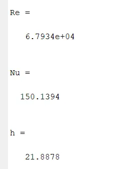

Physics /Mesh Setup

Geometry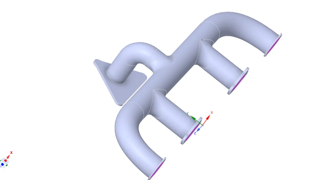

· Model imported into the space claim

· By using volume extract option, extracted the volume.

· Share topology between solid and fluid volume enabled (pink circles ensures the share topology is enabled)

· Created new component from both the volumes.

Mesh

Case1

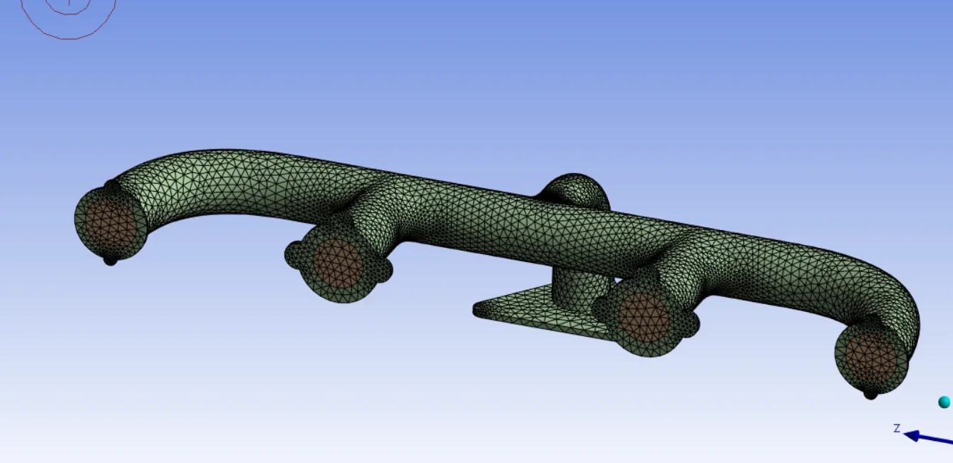
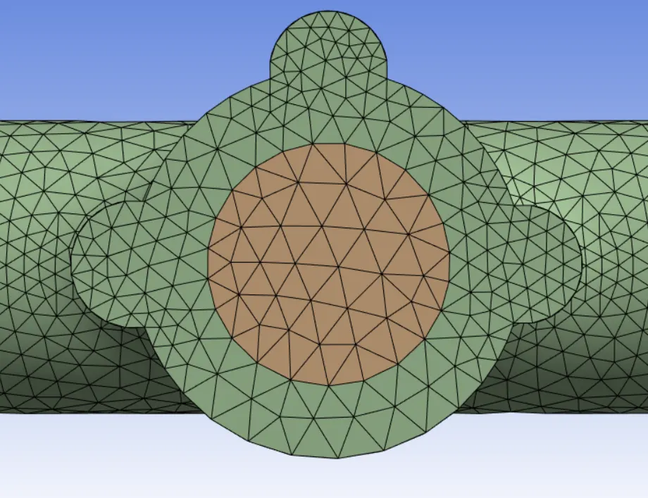
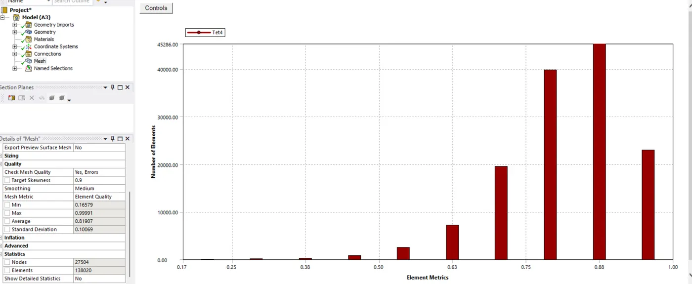
Case2

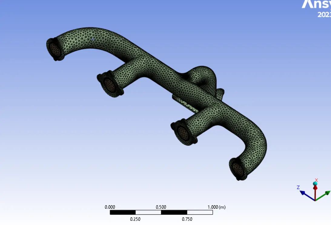
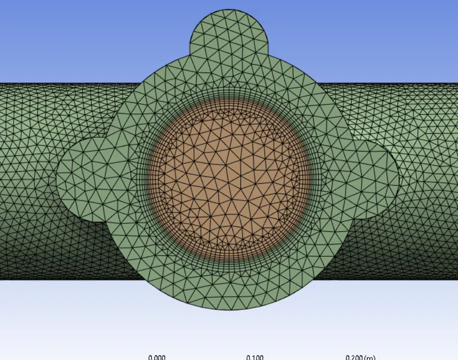
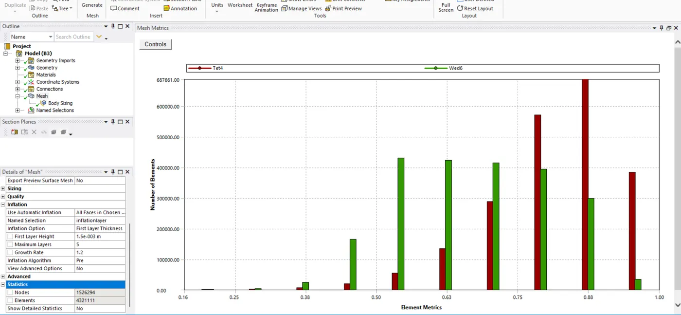
We have added inflation layer with first layer thickness 0.0015m as we calculated for Y+ value 30. Element size 0.05m.

Setting up of Physics,

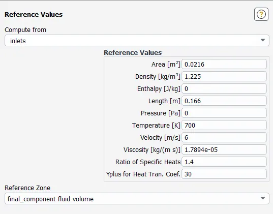
Refference Values

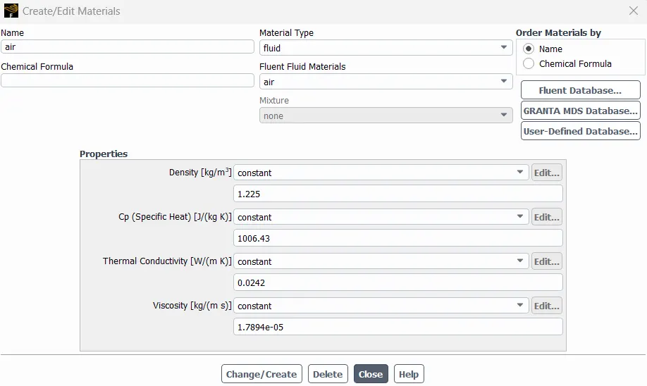
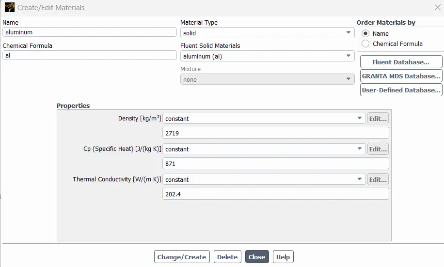
Material Properties

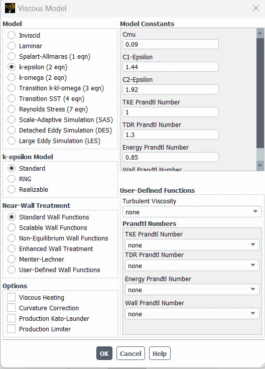
Viscous Model

Hybrid Initialization selected.

Analysis of all the cases

Case 1

1.1 Description of the case 1

Description	Values
Flow type	Steady state, pressure-based solver
Turbulence \ Viscous model	K- Epsilon
Inlet Velocity	6 m/s
Y+	-
Total Number of elements	138020
First layer Thickness	NA

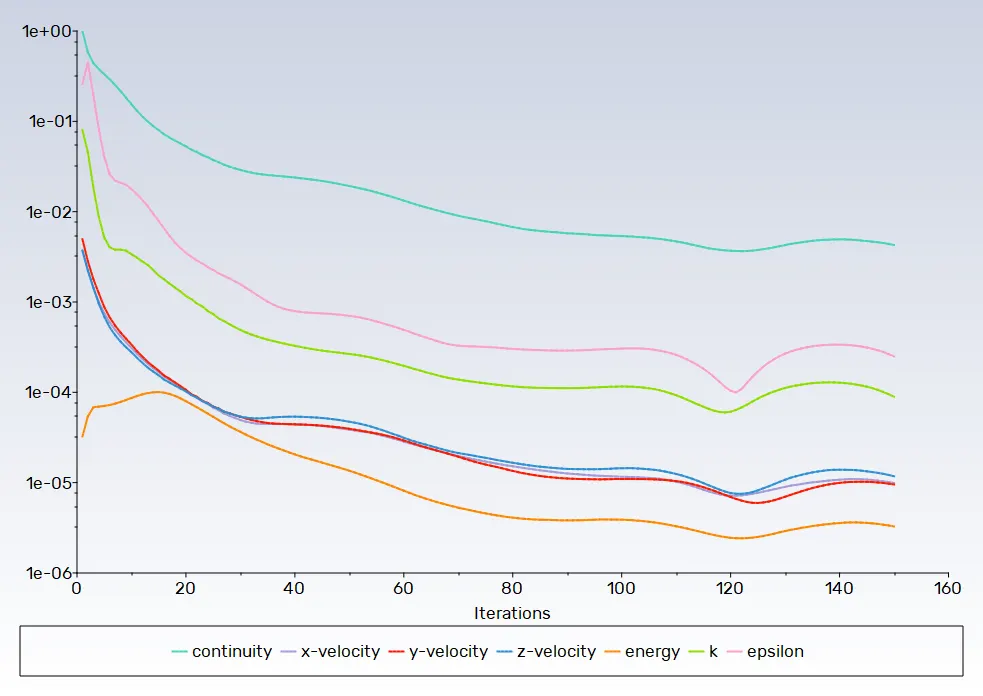
1.2 Line plot of Residual versus the iteration

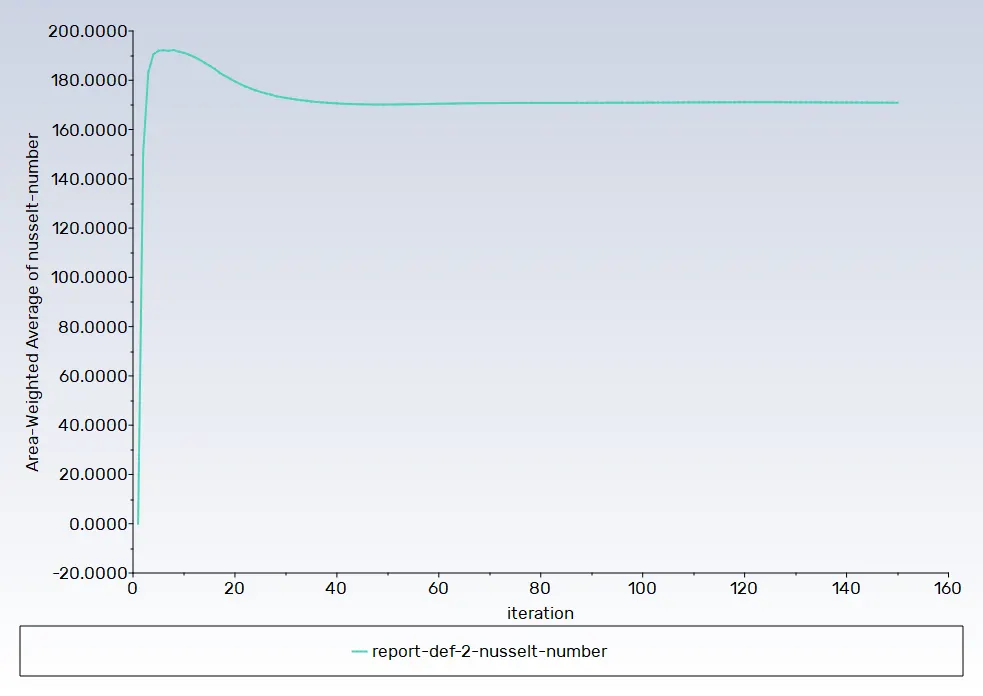
1.3 Line plot of Nusselt number versus the iteration

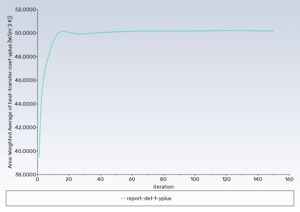
1.4 Line plot of Yplus based of heat transfer coefficient versus the iteration

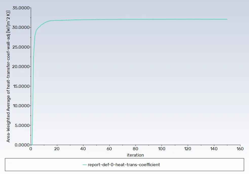
1.5 Line plot of heat transfer coefficient adjacent wall versus the iteration

1.6 Line plot of Temperature at outlet versus the iteration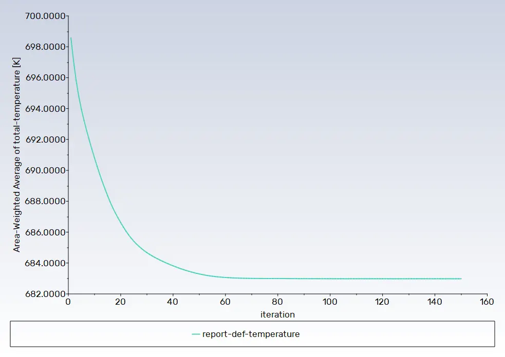

1.7 Result

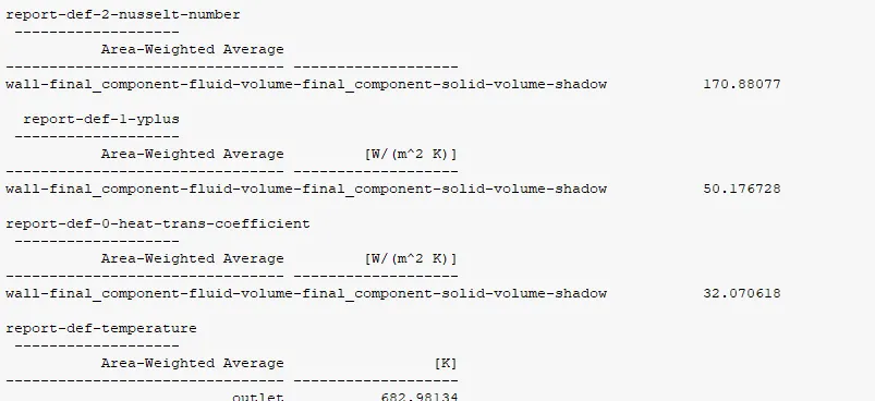
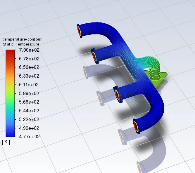
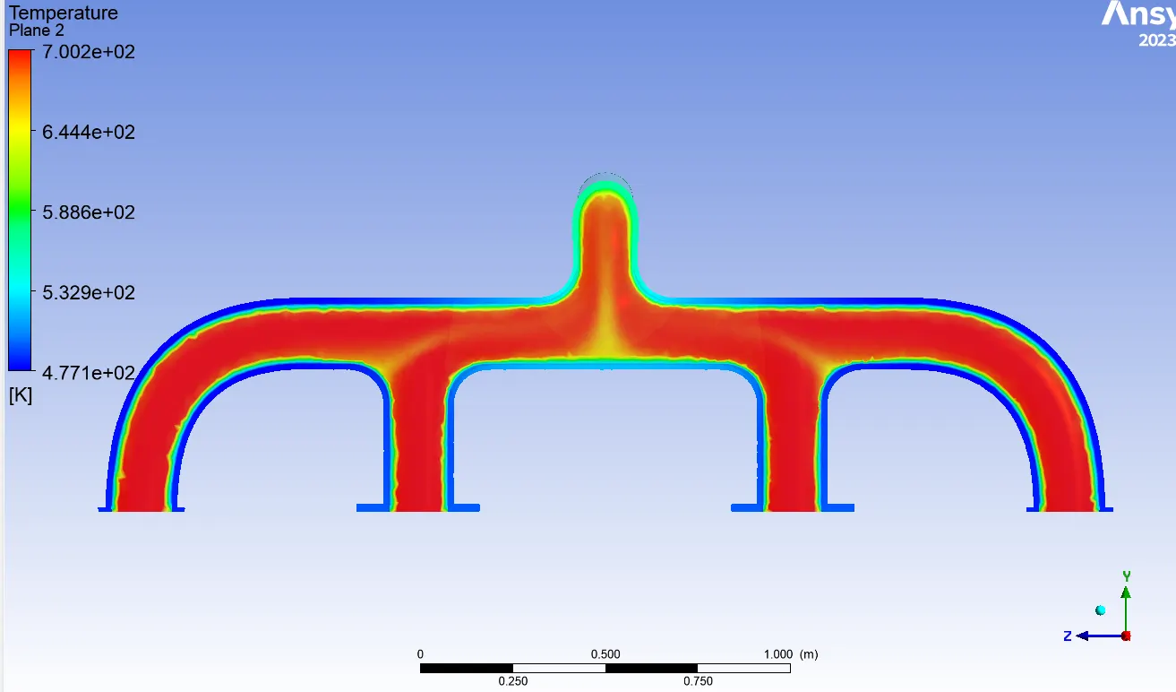
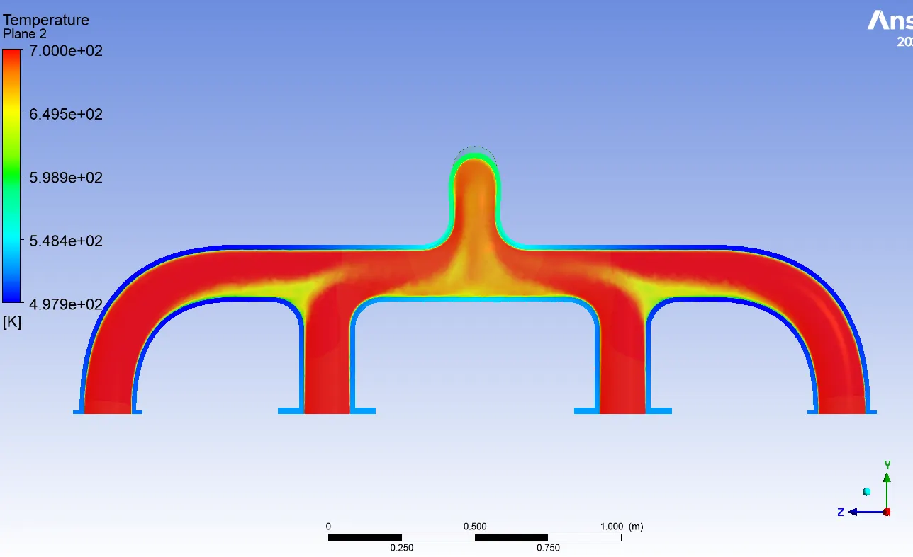
1.8 Contour plot of temperature

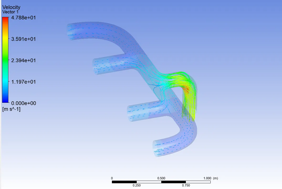
1.9 velocity stream line

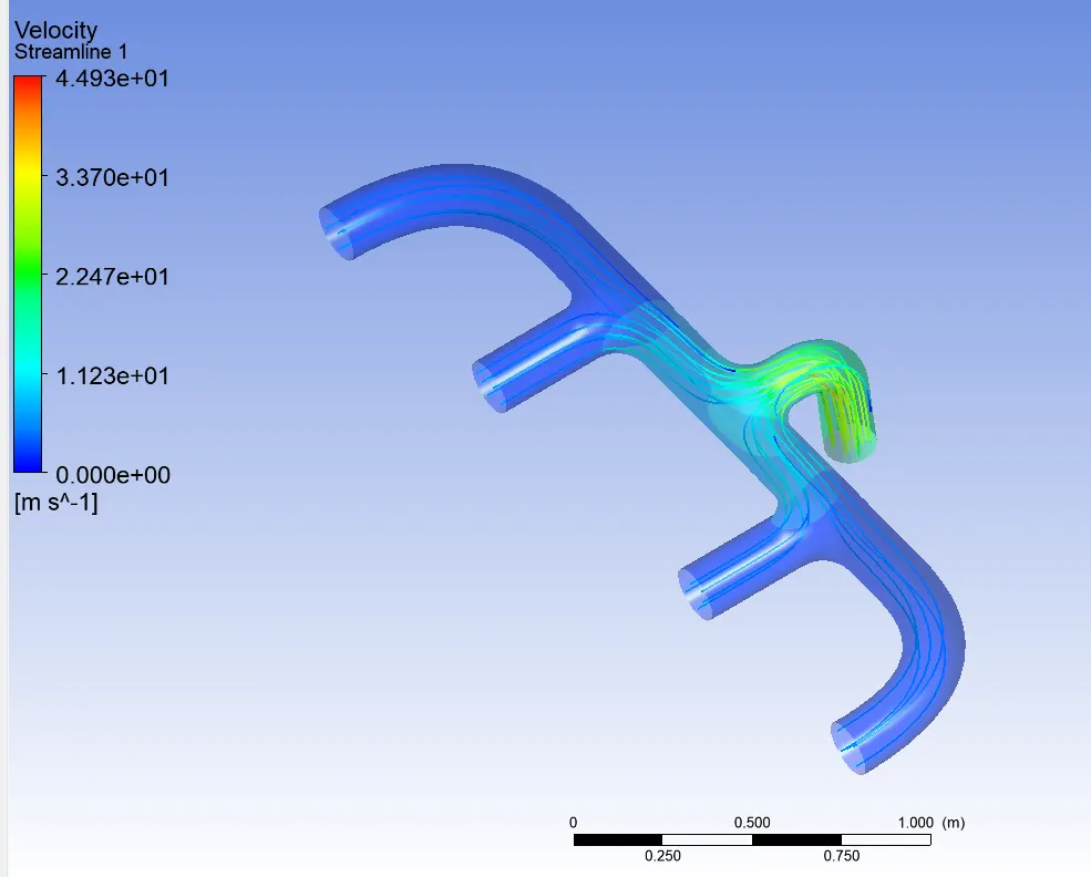
1.10 velocity contour

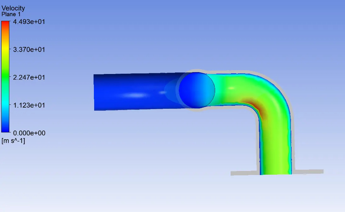
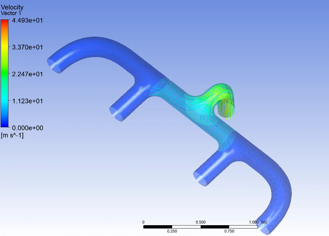
1.10 velocity vector

Case 2

2.1 Description of the case 2

Description	Values
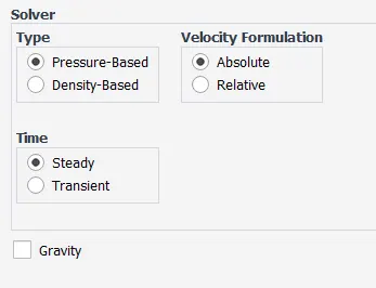
Flow type	Steady state, pressure-based solver
Turbulence \ Viscous model	K- Epsilon
Inlet Velocity	6 m/s
Y+	30
Total Number of elements	4321111
First layer Thickness	0.0015

2.2 Line plot of Residual versus the iteration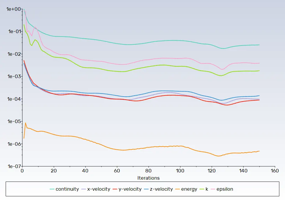

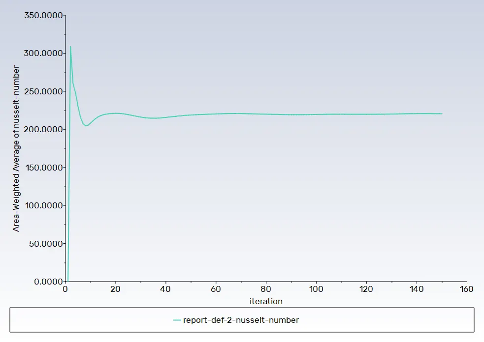
2.3 Line plot of Nusselt number versus the iteration

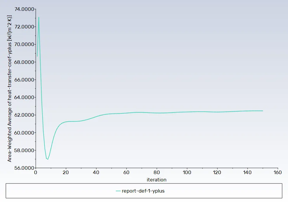
2.4 Line plot of Yplus based of heat transfer coefficient versus the iteration

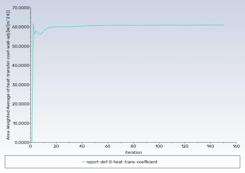
2.5 Line plot of heat transfer coefficient adjacent wall versus the iteration

2.6 Line plot of Temperature at outlet versus the iteration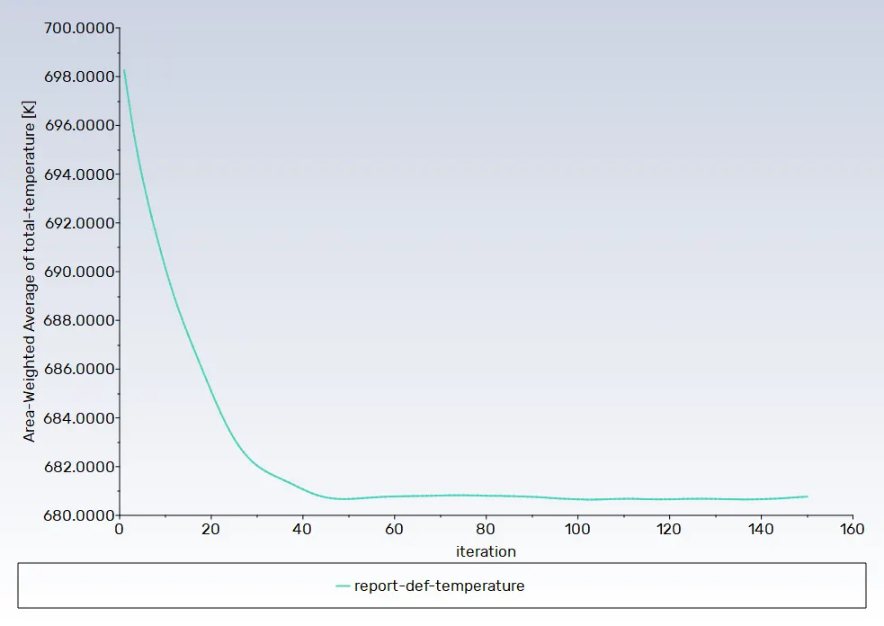

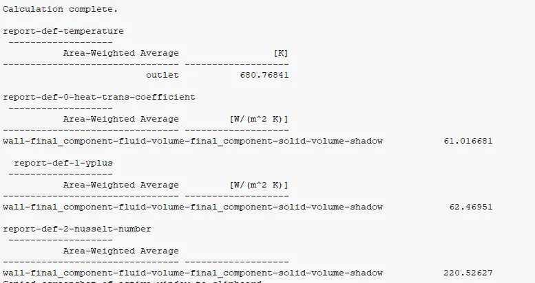
2.7 Result

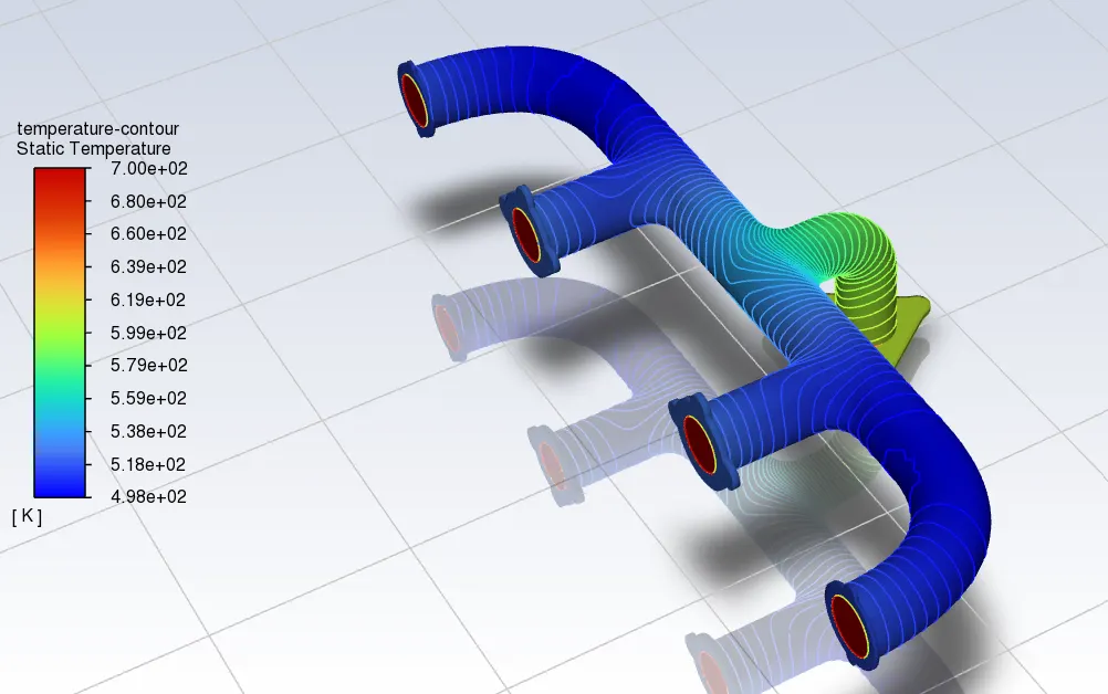
2.8 Contour plot of temperature

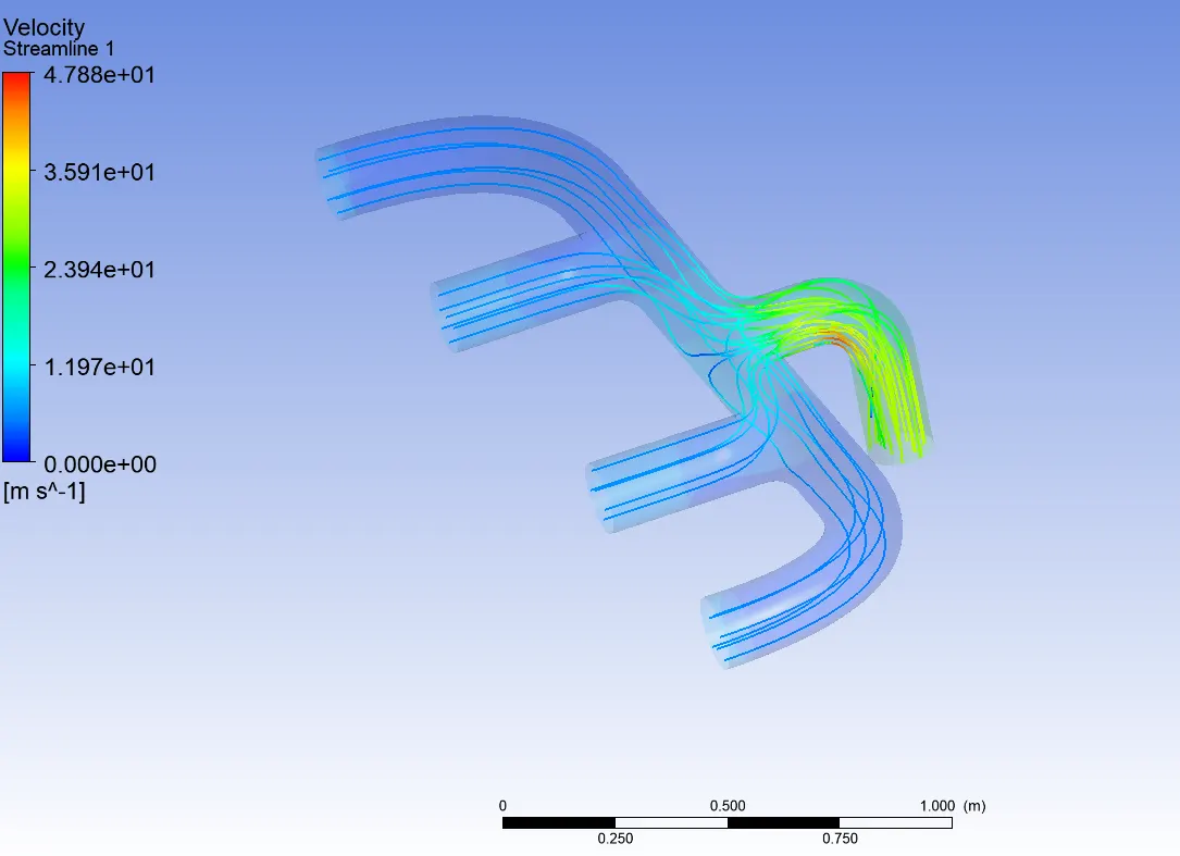
2.9 velocity stream line

2.10 velocity contour

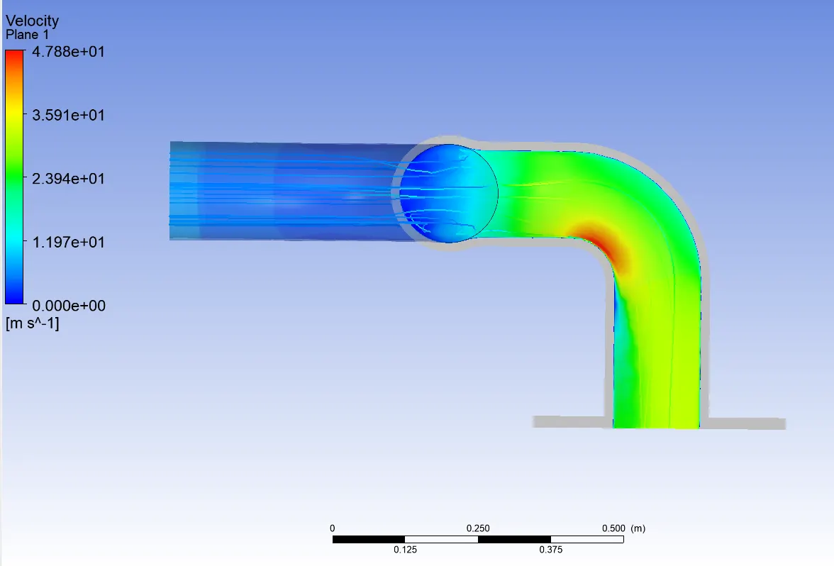
2.11 velocity vector

Conclusion

From the base line mesh which doesn't have inflation layer and from the Refined mesh we can conclude that The model with inflation layer can trap better wall adjacent values and conditions. Thus it signifies the importance of the inflation layer in capturing near-wall phenomenon.

As a fact we know that finer the mesh accurate the values are. The viscous models and solvers should be chosen according to the requirements. A good understanding of solvers and models is needed for CHT analysis.

Y plus values should be maintained depending on the solvers. Comparing the contours of temperature between the baseline mesh and refined mesh, we have observed that temperature is more accurate in case of refined mesh with an inflation layer

To get answer for how would you verify if the HTC predictions from the simulations are right? On what factors does the accuracy of the prediction depend on?

	HTC	Nusselt Number	Outlet temperature	HTC Error
Analytical	21.98	150	-	-
Base mesh	32.07	170	682 K	10.09
Refined Mesh	61.01	220	680 K	39.03

Using the above data the calculation done can be validated as the values are closer to the analytical values. There was no much of difference spotted comparing both cases, there was only a little change in the values obtained