To Analysis and Design of Steel Structures using TSD

Beams are long and slender structural elements, differing from truss elements in that they are called on to support transverse as well as axial loads. Their attachment points can also be more complicated than those of truss elements: they may be bolted or welded together, so the attachments can transmit bending moments or transverse forces into the beam. Beams are among the most common of all structural elements, being the supporting frames of airplanes, buildings, cars, people, and much else.

The nomenclature of beams is rather standard: as shown in Figure 1, L is the length, or span; b is the width, and hℎ is the height (also called the depth). The cross-sectional shape need not be rectangular, and often consists of a vertical web separating horizontal fllanges at the top and bottom of the beam (There is a standardized protocol for denoting structural steel beams; for instance W 8 × 40 indicates a wide-ffllange beam with a nominal depth of 8′′ and weighing 40 lb/ft of length)

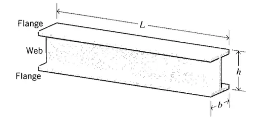
As will be seen in Modules 13 and 14, the stresses and deflections induced in a beam under bending loads vary along the beam's length and height. The first step in calculating these quantities and their spatial variation consists of constructing shear and bending moment diagrams, V(x) and M(x), which are the internal shearing forces and bending moments induced in the beam, plotted along the beam's length. The following sections will describe how these diagrams are made.

Free-body diagrams

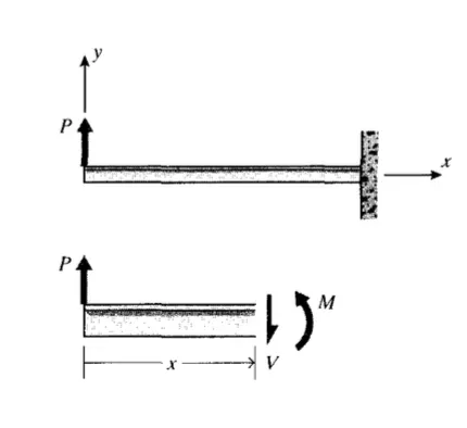
As a simple starting example, consider a beam clamped (\cantilevered") at one end and subjected to a load P at the free end as shown in Figure 2. A free body diagram of a section cut transversely at position x shows that a shear force V and a moment M must exist on the cut section to maintain equilibrium. We will show in Module 13 that these are the resultants of shear and normal stresses that are set up on internal planes by the bending loads. As usual, we will consider section areas whose normals point in the +x direction to be positive; then shear forces pointing in the +y direction on +x faces will be considered positive. Moments whose vector direction as given by the right-hand rule are in the +z direction (vector out of the plane of the paper, or tending to cause counterclockwise rotation in the plane of the paper) will be positive when acting on +x faces. Another way to recognize positive bending moments is that they cause the bending shape to be concave upward. For this example beam, the statics equations give:

Note that the moment increases with distance from the loaded end, so the magnitude of the maximum value of M compared with V increases as the beam becomes longer. This is true of most beams, so shear effects are usually more important in beams with small length-to-height ratios.

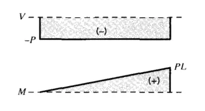
As stated earlier, the stresses and defflections will be shown to be functions of V and M, so it is important to be able to compute how these quantities vary along the beam's length. Plots of V(x) and M(x) are known as shear and bending moment diagrams, and it is necessary to obtain them before the stresses can be determined. For the end-loaded cantilever, the diagrams shown in Figure 3 are obvious from Eqns. 4.1.1 and 4.1.2.

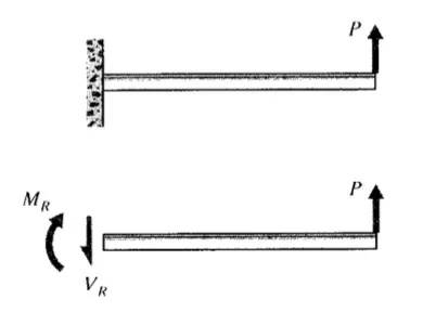
It was easiest to analyze the cantilevered beam by beginning at the free end, but the choice of origin is arbitrary. It is not always possible to guess the easiest way to proceed, so consider what would have happened if the origin were placed at the wall as in Figure 4. Now when a free body diagram is constructed, forces must be placed at the origin to replace the reactions that were imposed by the wall to keep the beam in equilibrium with the applied load. These reactions can be determined from free-body diagrams of the beam as a whole (if the beam is statically determinate), and must be found before the problem can proceed. For the beam of Figure 4:

∑Fy=0=−VR+P⇒VR=P∑=0

The shear and bending moment at x are then

V(x)=VR=P=constant

This choice of origin produces some extra algebra, but the V(x) and M(x) diagrams shown in Figure 5 are the same as before (except for changes of sign): V is constant and equal to P, and M varies linearly from zero at the free end to PL at the wall.

Distributed loads

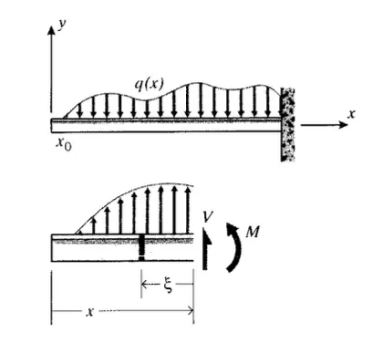
Transverse loads may be applied to beams in a distributed rather than at-a-point manner as depicted in Figure 6, which might be visualized as sand piled on the beam. It is convenient to describe these distributed loads in terms of force per unit length, so that q(x) would be the load applied to a small section of length dx by a distributed load q(x). The shear force V(x) set up in reaction to such a load is

If the boundary condition indicates that the beam is fixed in a specific direction, then an external reaction in that direction can exist at the location of the boundary condition. For example, if a beam is fixed in the y-direction at a specific point, then a transverse (y) external reaction force may develop at that point. Likewise, if the beam is fixed against rotation at a specific point, then an external reaction moment may develop at that point.

Based on the above discussion, we can see that a fixed boundary condition can develop axial and transverse reaction forces as well as a moment. Likewise, we see that a pinned boundary condition can develop axial and transverse reaction forces, but it cannot develop a reaction moment.

Notice the Free boundary condition in the table above. This boundary condition indicates that the beam is free to move in every direction at that point (i.e., it is not fixed or constrained in any direction). Therefore, a constraint does not exist at this point. This highlights the subtle difference between a constraint and a boundary condition. A boundary condition indicates the fixed/free condition in each direction at a specific point, and a constraint is a boundary condition in which at least one direction is fixed.

Shear Force and Bending Moment

To find the shear force and bending moment over the length of a beam, first solve for the external reactions at each constraint. For example, the cantilever beam below has an applied force shown as a red arrow, and the reactions are shown as blue arrows at the fixed boundary condition.

The external reactions should balance the applied loads such that the beam is in static equilibrium. After the external reactions have been solved for, take section cuts along the length of the beam and solve for the internal reactions at each section cut. (The reaction forces and moments at the section cuts are called internal reactions because they are internal to the beam.) An example section cut is shown in the figure below:

When the beam is cut at the section, either side of the beam may be considered when solving for the internal reactions. The side that is selected does not affect the results, so choose whichever side is easiest. In the figure above, the side of the beam to the right of the section cut was selected. The selected side is shown as the blue section of beam, and section shown in grey is ignored. The internal reactions at the section cut are shown with blue arrows. The reactions are calculated such that the section of beam being considered is in static equilibrium.

• CSI SAFE (Slab Analysis by the Finite Element Method) is the best tool for designing concrete slabs and foundations.
• SAFE provide easiness to engineer towards the safe design of structures with powerful tools like draw, analyze, design and detailing etc.
• Laying out models is quick and efficient way with the user-friendly drawing tools, or user can import model layouts from AutoCAD or loading conditions from other software’s like CSI ETABS and CSI SAP2000.

PROCEDURE:

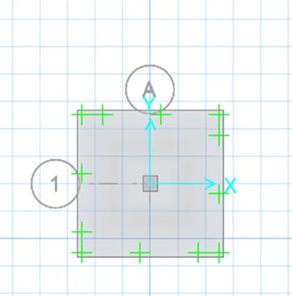
Open the SAFE Application and select New Model followed by Input Settings, Units was selected as Metric and Code IS 456-2000.

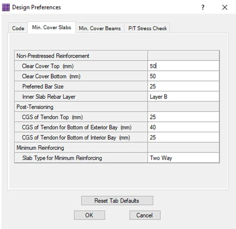
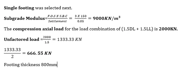
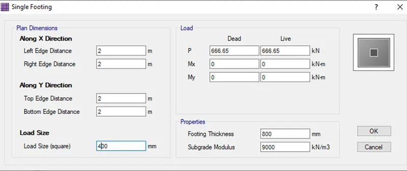
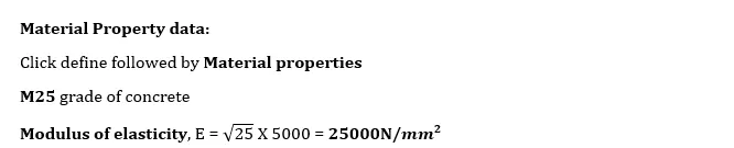
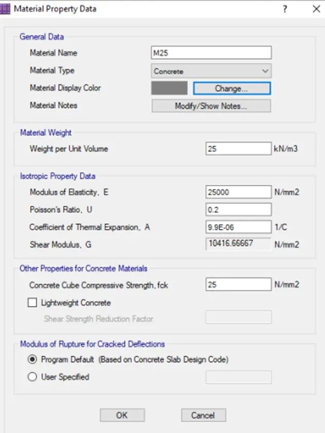
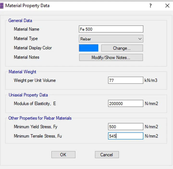
Fe 500 Rebar was added next as shown

Slab properties was defined next as shown

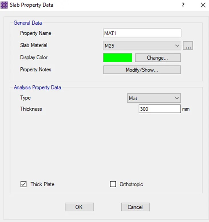
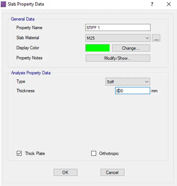
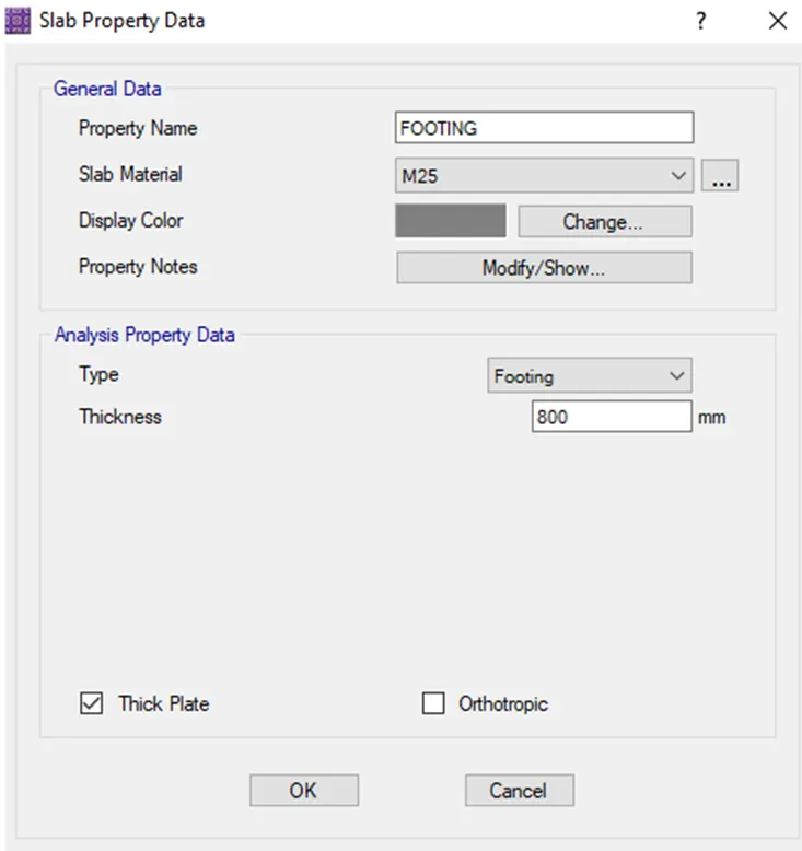
Soil properties was added next as shown

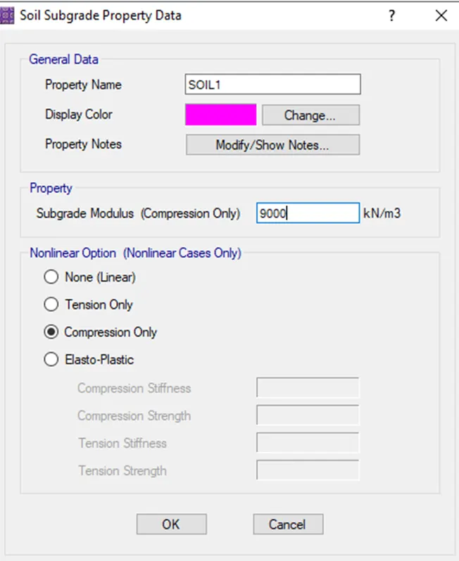
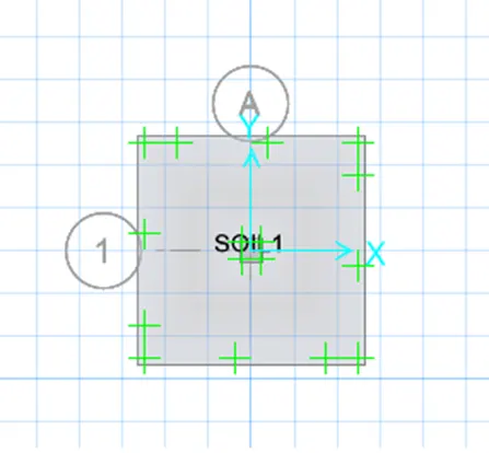
In order to open the properties right click on the footing

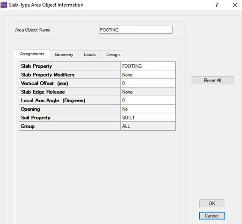
Load properties:

Both dead and live load patterns was defined next

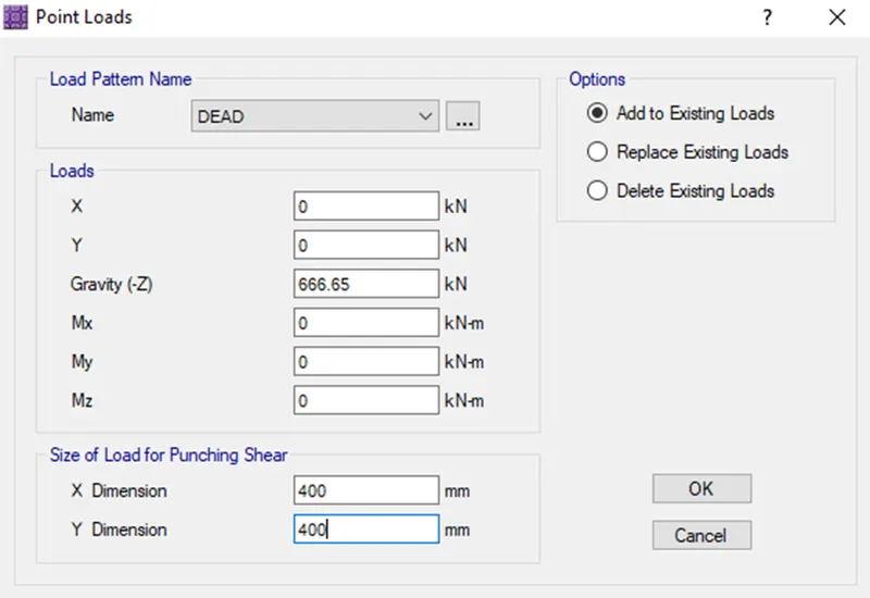
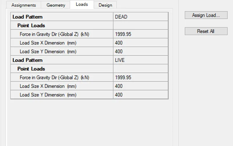
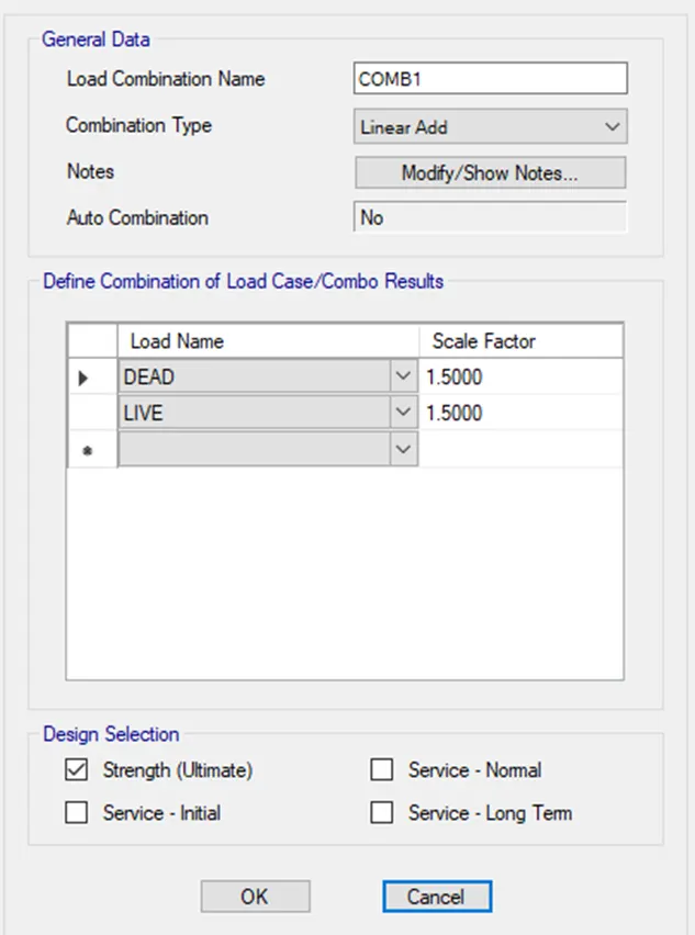
Load case combination was defined next

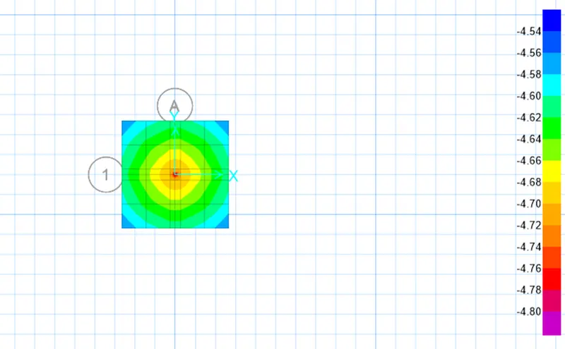
Analysis was performed next

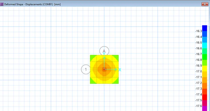
Design strip was added next and Analysis was performed.

The slab design is as shown below

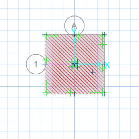
Result:

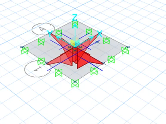
Isolated footing was designed using SAFE