Supervised Learning - Prediction

Supervised Learning

Prediction

1. Gradient Descent

The gradient descent in python using mean square error as loss function on the following data set:

x = [0,1,2,3,4]

y = [1,2,3,4,5]

Theory:

`J = (1/n) sum(y(i) - (mx(i) + b))^2`

x(i) are the input

m and b are the weights

mx(i)+b is the predicted output and y(i) is the actual value

Differentiating the loss function J with respect to m and b, we get

`(dJ)/(dm) = (2/n) sum - x(i)(y(i) - (mx(i) + b))`

`(dJ)/(db) = (2/n) sum - (y(i) - (mx(i) + b))`

`m = m - alpha*(dJ)/(dm)`

`b = b - alpha*(dJ)/(db)`

`alpha` is the learning rate, i.e how large a step the gradient takes.

Python Code:

import numpy as np
import matplotlib.pyplot as plt
from scipy.optimize import curve_fit
from statistics import mean

#Initialising data
y = [1,2,3,4,5]
x = [0,1,2,3,4]

#fit function y = mx+b
n = len(y) #number of elements

#Initialising parameters
m = 0
b = 0

#Learning rate alpha
alp = 0.0008

#Cost function
J = 9e9
tol = 1e-4 #Error tolerance
iter = 1 #Iterations

while (J>tol): #If error is greater than tolerance while loop is executed

term1 = []; #Empty array initialised
d_m = []; #Gradient of parameter m
d_b = []; #Gradient of parameter b

for i in range(0,n):
term1.append(pow(y[i]-m*x[i]-b,2))
d_m.append(-x[i]*(y[i]-m*x[i]-b))
d_b.append(-y[i]+m*x[i]+b)

print("nNumber of iterations:",iter)
iter = iter+1
J = (1/n)*sum(term1)
print("nError:",J)
print("nParameters:")
print("nm value:",m)
print("nb value:",b)
m = m - alp*(2/n)*sum(d_m)
b = b - alp*(2/n)*sum(d_b)

Code Explanation:

Necessary libraries are imported to execute the program

import numpy as np
import matplotlib.pyplot as plt
from scipy.optimize import curve_fit
from statistics import mean

Initial data and parameters are initialized

#Initialising data
y = [1,2,3,4,5]
x = [0,1,2,3,4]

#fit function y = mx+b

n = len(y) #number of elements

#Initialising parameters
m = 0
b = 0

#Learning rate alpha
alp = 0.0008

Main body

while (J>tol): #If error is greater than tolerance while loop is executed
	term1 = []; #Empty array initialised
	d_m = []; #Gradient of parameter m 
	d_b = []; #Gradient of parameter b
	for i in range(0,n):
		term1.append(pow(y[i]-m*x[i]-b,2))
		d_m.append(-x[i]*(y[i]-m*x[i]-b))
		d_b.append(-y[i]+m*x[i]+b)

If the condition J>tol is true, then the while loop will be executed.

for i in range(0,n):
		term1.append(pow(y[i]-m*x[i]-b,2))
		d_m.append(-x[i]*(y[i]-m*x[i]-b))
		d_b.append(-y[i]+m*x[i]+b)

Inside the while loop, there is a for loop which fetches each value present in x and y and calculates the error and change in the loss function with respect to the parameters m and b

print("nNumber of iterations:",iter)
	iter = iter+1
	J = (1/n)*sum(term1)
	print("nError:",J)
	print("nParameters:")
	print("nm value:",m)
	print("nb value:",b)
	m = m - alp*(2/n)*sum(d_m)
	b = b - alp*(2/n)*sum(d_b)

After exiting the for loop, the sum of the terms are calculated and this process keeps repeating till the error is lesser than the given tolerance value

Result:

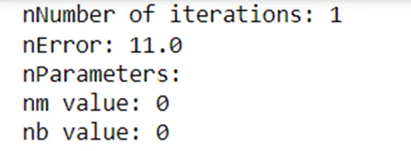
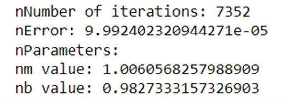
For a learning rate of 0.0008, it takes 7352 iterations for the error to be lesser than the tolerance and the m and b values are found to be 1.006 and 0.982 which are mathematically correct.

2. Difference between L1 & L2 Gradient descent method

L1 Mean absolute error: finds the mean of the absolute difference between the predicted and actual value. It is good for data set with little or no outliers. However, it needs more complicated tools such as linear programming to calculate the gradients of the parameters.

L2 Mean squared error: Finds the mean of the square of the difference between the predicted and actual value. It is good for data set with outliers, however returns an error in different units. Due to its mathematical properties, it is easier to calculate the gradients of the parameters. The squaring means that larger mistakes result in more error than smaller mistakes, meaning that the model is punished for making larger mistakes.

Finding the root of the mean squared error, i.e. using root mean square error bring the error term to match with the data set in terms of units.

3. Different loss functions for regression

• Mean square error
• Mean absolute error
• Huber loss
• Log cosh loss
• Quantile loss

1. Mean Square Error or L2 Loss:
Mean Square Error (MSE) is the most commonly used regression loss function. MSE is the sum of squared distances between our target variable and predicted values.

2. Mean Absolute Error, L1 Loss:
Mean Absolute Error (MAE) is another loss function used for regression models. MAE is the sum of absolute differences between our target and predicted variables. So it measures the average magnitude of errors in a set of predictions, without considering their directions. (If we consider directions also, that would be called Mean Bias Error (MBE), which is a sum of residuals/errors). The range is also 0 to ∞.

3. Huber Loss:
Huber loss is also called Smooth Mean Absolute Error. This loss function is less sensitive to outliers in data than the squared error loss. It’s also differentiable at 0. It’s basically absolute error, which becomes quadratic when error is small. How small that error has to be to make it quadratic depends on a hyperparameter, 𝛿 (delta), which can be tuned. Huber loss approaches MSE when 𝛿 ~ 0 and MAE when 𝛿 ~ ∞ (large numbers.)

4. Log-Cosh Loss
Log-cosh is another function used in regression tasks that’s smoother than L2. Log-cosh is the logarithm of the hyperbolic cosine of the prediction error.

5. Quantile Loss
In most of the real world prediction problems, we are often interested to know about the uncertainty in our predictions. Knowing about the range of predictions as opposed to only point estimates can significantly improve decision making processes for many business problems.

Quantile loss functions turn out to be useful when we are interested in predicting an interval instead of only point predictions. Prediction interval from least square regression is based on an assumption that residuals (y — y) have constant variance across values of independent variables. We can not trust linear regression models which violate this assumption. We can not also just throw away the idea of fitting linear regression model as baseline by saying that such situations would always be better modeled using non-linear functions or tree based models. This is where quantile loss and quantile regression come to rescue as regression based on quantile loss provides sensible prediction intervals even for residuals with non-constant variance or non-normal distribution.

4. Importance of learning rate

Let F be a function that determines the error between the data set and the predicted values. The predicted values depend on two parameters m, and c. Gradient descent is a method to determine the values of the parameters for which F returns the least value.

Learning rate is an important factor that determines how fast the function parameter approaches a nominal value. Gradient descent is a method to determine the values of the function parameters for which the function returns the minimum error.

`F = 1/(2n) * sum_(i=1)^n ((mx_i + c) - Y_i)^2`

`m = m - alpha((dF)/(dm))`

`c = c - alpha((dF)/(dc))`

Giving a high learning rate will cause the function to overshoot beyond its lowest value and will never reach its lowest value or will oscillate before arriving at one.

Giving a low learning rate will cause the function to approach the lowest value very slowly leading to a high number of iterations.

5. How to evaluate linear regression

Linear regression is a regression model that uses a straight line to describe the relationship between variables. It finds the line of best fit through your data by searching for the value of the regression coefficient(s) that minimizes the total error of the model.

There are two main types of linear regression:

• Simple linear regression uses only one independent variable
• Multiple linear regression uses two or more independent variables

In this step-by-step guide, we will walk you through linear regression in R using two sample datasets.

There are three error metrics that are commonly used for evaluating and reporting the performance of a regression model; they are:

• Mean Squared Error (MSE)
• Root Mean Squared Error (RMSE)
• Mean Absolute Error (MAE)

There are many other metrics for regression, although these are the most commonly used.

Linear regression can be evaluated by determining how good the fit is, i.e. what is the error between the predicted value and the data set.

R-squared:

Assume function f(x) to satisfy the data points (x1,y1), (x2,y2).. and so on.

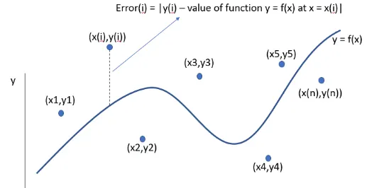
Sum of square error SSE

`SSE = sum_(i=1)^n (y(i) - f(x(i)))^2`

If the proposed equation is an nth degree polynomial

f(x)=A1+A2⋅x+A3⋅x2+..+A n⋅xn-1">f(x)=A1+A2⋅x+A3⋅x2+..+A n⋅xn−1f(x)=A1+A2⋅x+A3⋅x2+..+A n⋅xn-1

Differentiating the SSE with each coefficient and equating it to zero will return us the value of the coefficient for which the error is minimum.

Solving the multiple systems of equations we can get the value of the coefficients.

This is the least square error method.

R-square:

`R" square" = (SSR)/(SST)`, where

`SST = SSE + SSR`

SSR stands for the sum of the square of the regression and is equal to the square of the difference between the value of the fitting function at the given point and the mean of the data set.

`SSR = sum_(i=1)^N(f(x(i)) - M)^2`, where M is the arithmetic mean of the given data set.

6. Difference between Multiple and Adjusted coefficient of determination

Coefficient of determination:

In statistics, the coefficient of determination, denoted `R^2 or r^2` and pronounced "R squared", is the proportion of the variation in the dependent variable that is predictable from the independent variable(s).

It is a statistic used in the context of statistical models whose main purpose is either the prediction of future outcomes or the testing of hypotheses, on the basis of other related information. It provides a measure of how well observed outcomes are replicated by the model, based on the proportion of total variation of outcomes explained by the model.

Multiple R squared is simply a measure of Rsquared for models that have multiple predictor variables. Therefore it measures the amount of variation in the response variable that can be explained by the predictor variables. The fundamental point is that when you add predictors to your model, the multiple Rsquared will always increase, as a predictor will always explain some portion of the variance.

Adjusted R squared controls against this increase, and adds penalties for the number of predictors in the model. Therefore it shows a balance between the most parsimonious model, and the best fitting model. Generally, if you have a large difference between your multiple and your adjusted Rsquared that indicates you may have overfit your model.