Supervised Learning - Classification

Supervised Learning

Classification

1. KNN on Surface Defects in Stainless Steel Plates

K-Nearest Neighbors is a supervised machine learning algorithm that classifies a data point based on how its neighbors are classified. It classifies new cases based on feature similarity measures.

KNN algorithm

K in the KNN algorithm is a parameter that refers to the number of nearest neighbors to include in the majority voting process. It is important to choose the right value of k in order to attain high model accuracy and this is achieved by parameter tuning.

KNN is used for data that is labeled, small in size, and noise-free.

KNN algorithm calculates the distance between two points using the Euclidean formula.

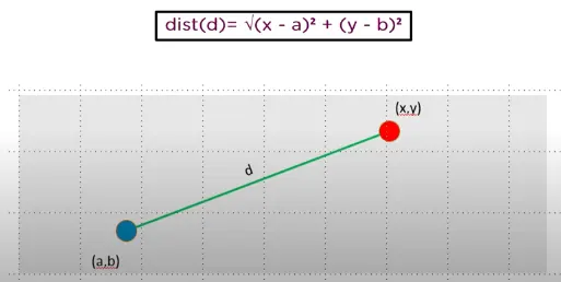
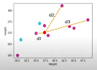
It'll calculate the distance between the unknown data point and all the points in the dataset, and based on the distance value, it'll classify the data point.

Code:

# Importing the libraries
import pandas as pd
import numpy as np
import matplotlib.pyplot as plt
import seaborn as sns
from sklearn.model_selection import train_test_split
from sklearn.neighbors import KNeighborsClassifier
from sklearn.metrics import accuracy_score
from sklearn.metrics import plot_confusion_matrix

# Importing the dataframe
df = pd.read_csv('C:/Users/Shivaani/Desktop/Skill-Lync/Machine Learning Fundamentals in Depth/Week_8 Programs/faults.csv')
df.head()

# Size of data
df.shape

# Print column names of data
df.columns

# To check for datatype and presence of null value for each column
df.info()

# Last seven columns are type of error classification
label_columns = df.columns.values[-7:]
label_columns

# Assigning the error classification values to variable targets
targets = (df.iloc[:,-7:]==1).idxmax(1)
targets

# Dropping the 7 error classification columns and retaining only targets
dataset = df.drop(label_columns,axis=1)

# Creating a new column 'target' with all classification values
dataset['target'] = targets
dataset

# Printing count of each type of error
dataset.target.value_counts()

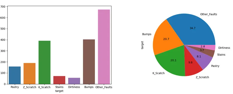
# Visualising the distribution of each error using histogram and pie chart
fig, ax = plt.subplots(1,2,figsize=(15,6))
sns.countplot(x='target',data=dataset, ax=ax[0])
dataset['target'].value_counts().plot.pie(autopct = '%.1f', ax=ax[1])

# Visualising the correlation among each dataset feature
plt.figure(figsize=(10,10))
sns.heatmap(dataset.corr(),annot=False)

# Dropping features with high correlation to others
dataset=dataset.drop('TypeOfSteel_A400',axis=1)
dataset=dataset.drop('X_Minimum',axis=1)
dataset=dataset.drop('Y_Minimum',axis=1)

# Assigning feature column values to x
x = dataset.iloc[:,0:24]

# Assingning target column values to y 
y = dataset.iloc[:,24]

# Splitting the dataset to training and testing sets
x_train,x_test,y_train,y_test = train_test_split(x,y,test_size = 0.2, random_state = 0)

# KNN model
knn = KNeighborsClassifier(n_neighbors= 19)
knn.fit(x_train,y_train)
classfier = knn.fit(x_train,y_train)
print("nKNN accuracy:",knn.score(x_test,y_test))
plot_confusion_matrix(classfier,x_test,y_test,labels=None, sample_weight=None, normalize=None)
plt.show()

Result:

Visualising countplot and pieplot:

Heatmap:

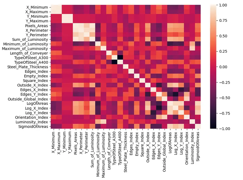
With the help of a heatmap, we can conclude that there is a high correlation between X minimum and X maximum, Y minimum and Y maximum, and type of steel A300 and A400.

Accuracy of model

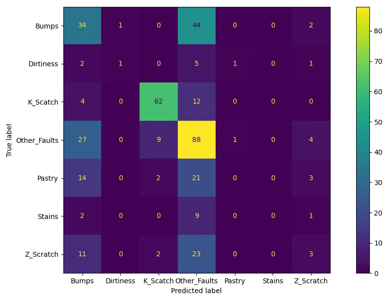
The KNN model has an accuracy of 48.32%.

Confusion Matrix:

2. Pros and Cons of KNN

Pros:

• It is a simple Machine Learning algorithm and easy to understand.
• kNN can be used for classification and regression.
• It can be used for multi-class problem.
• It provides a variety of distance criteria to choose from: Euclidean Distance Hamming Distance Manhattan Distance Minkowski Distance

Cons:

• It is difficult to choose the optimal number of neighbors to be consider while classifying the new data entry.
• K-NN inherently has no capability of dealing with missing value problem.
• k Nearest Neighbor has calculate the proximity between each neighbors for every single value in the dataset. For large daasets its computation cost increases.