Medical Insurance Dataset - Statistical Analysis
Project 1
Using the existing dataset of medical insurance data, we can understand the relationships between the features and the target variable and make predictions on new data.
1. Analyzing the Data
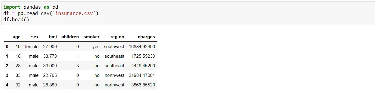
The data consists of the following columns:
This dataset is used to predict charges (insurance costs) based on other features. Therefore, this is a supervised learning problem where charges is the dependent variable and the others are independent variables.
2. Estimating the Minimum Sample Size
The minimum sample size n required for 99�curate predictions can be calculated using the formula:
n = (Z^2 * p * (1-p)) / e^
Since, the proportion p of the population is unknown, it can be estimated as 0.5. With a precision of 0.02 and Z = 2.576, we get:
n = (2.576^2 * 0.5 * (1-0.5)) / 0.02^2 = 4147.38
So, the minimum sample size required for 99�curate predictions with a precision of 0.02 is approximately 4148.
3. Data Cleaning
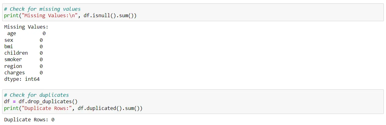
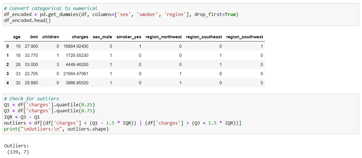
Interpretation:
There are no missing values in the dataset.
There are no duplicate rows in the dataset.
Categorical variables sex, smoker, and region are converted to numerical values.
There are 139 outliers in the charges column based on the IQR method. This suggests a significant number of data points have charges much higher or lower than the typical range.
4. Checking if Sex and Smoking are Statistically Independent
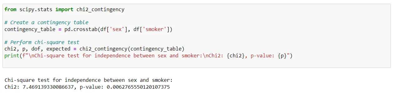
Interpretation:
The chi-square test results in a p-value of approximately 0.0062.
Since the p-value is less than 0.05, we reject the null hypothesis and conclude that sex and smoker are not independent. There is a statistically significant relationship between sex and smoker.
5. Checking Independence of Regressor Variables
Interpretation:
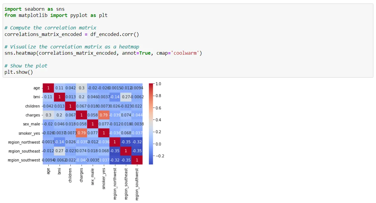
The correlation matrix shows the pairwise correlation between variables.
None of the independent variables have extremely high correlations with each other, suggesting they are mostly independent.
'smoker' has a high correlation with 'charges' (0.79), indicating a strong relationship between smoking status and insurance charges.
6. Checking Dependency between Response and Regressor
Interpretation:
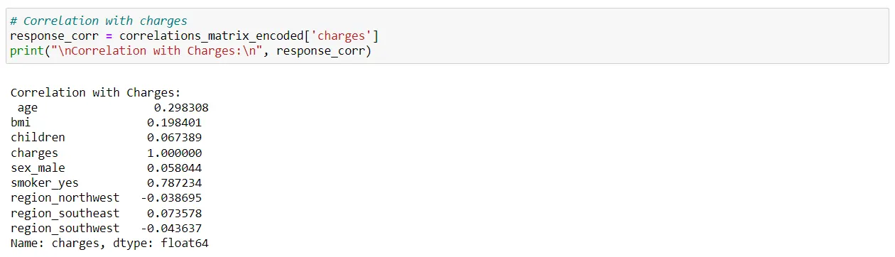
'smoker' has the highest positive correlation with 'charges' (0.787), followed by age (0.298) and bmi (0.198).
'sex_male' has a correlation with 'charges' (0.05), indicating male might have slightly higher charges than female.
The correlations suggest that smoking status, age, and BMI are significant predictors of insurance charges.
7. Predicting the Regression Line
Interpretation:
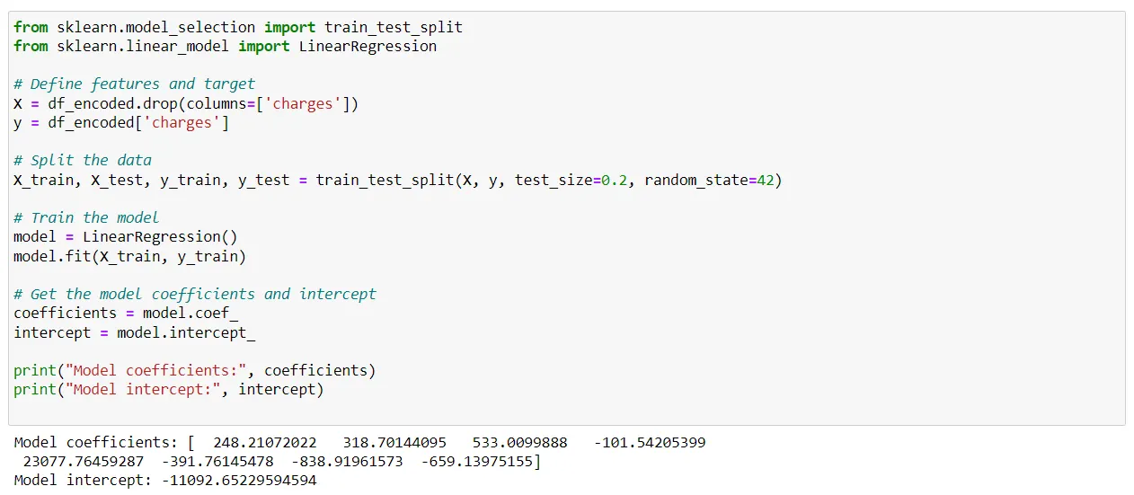
The regression model has been trained with the coefficients for each feature.
The intercept is -11092.51, which represents the baseline insurance charge when all features are zero.
8. Predicting the Accuracy of Regression Model
Interpretation:
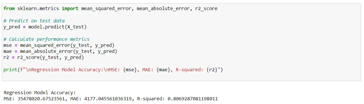
Mean Squared Error (MSE) is approximately 35,478,020.
Mean Absolute Error (MAE) is approximately 4,177.04.
R-squared value is 0.806, indicating that about 80.6% of the variance in charges can be explained by the model. This suggests a good fit.
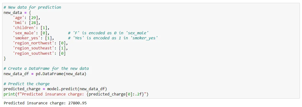
9. Predicting Insurance Charge for Age = 29, Sex = F, BMI = 28, Children = 1, Smoke = Yes, Region = southeast
Interpretation:
The predicted insurance charge for a 29-year-old female, with a BMI of 28, 1 child, who smokes, and lives in the southeast region is approximately 27,800.95
10. Percentage of Error in Regression Model

Interpretation:
The Mean Absolute Percentage Error (MAPE) is approximately 41.40%, indicating that on average, the predictions are off by about 41.40% from the actual values.
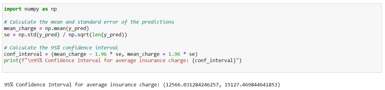
11. 95% Confidence Interval for Average Charge Insurance
Interpretation:
The 95% confidence interval for the average insurance charge is approximately (12,566.03, 15,127.47). This means we can be 95% confident that the true mean insurance charge lies within this interval.