Implementing Clustering and Predicting the Class of Car from "Car Dataset"
Implementing Clustering and Predicting the Class of Car from "Car Dataset"
Importing libraries
import pandas as pd
import numpy as np
import seaborn as sn
from sklearn.preprocessing import LabelEncoder
from sklearn.preprocessing import  MinMaxScaler
from sklearn.linear_model import LinearRegression
from sklearn.ensemble import RandomForestRegressor
from sklearn.model_selection import train_test_split
import matplotlib.pyplot as plt
import sklearn.cluster as cluster
from sklearn.cluster import KMeans
from sklearn.decomposition import PCA
import sklearn.metrics as metrics
from sklearn.tree import DecisionTreeClassifier
from sklearn.ensemble import RandomForestClassifier
from sklearn.linear_model import LinearRegression
from sklearn.neighbors import KNeighborsClassifier
from sklearn.svm import SVC
from sklearn.metrics import confusion_matrix
from sklearn.metrics import classification_report
Importing the dataset
df=pd.read_csv("cars.csv")
df.head()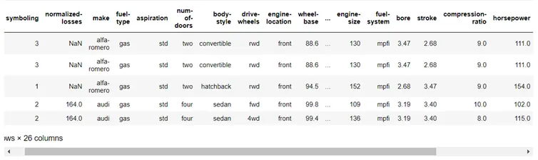
Information on the dataset
df.info()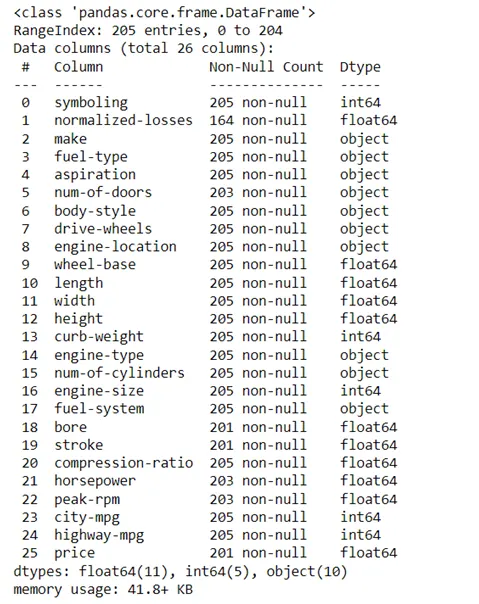
Replacing "?" with NaN values
df.replace("?", np.nan, inplace = True)
Saving the changes to a new dataset "cars_dataset"
df.to_csv("cars_dataset.csv", index=False)Importing the new dataset
df2 = pd.read_csv('cars_dataset.csv')
df2.head()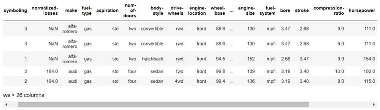
Count of all the null values
df2.isnull().sum()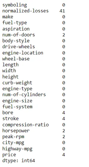
Observation:
We can see that the "?" were replaced by NaN. Now this can be easily replaced by values.
Replacing null values of normalized-loss, bore, stroke, horespower, peak-rpm with the median of their respective columns
a_n = df2["normalized-losses"].astype("float").median(axis=0)
print("Average of normalized-losses: ", a_n)

a_b = df2['bore'].astype('float').median(axis=0)
print("Average of bore: ", a_b)

a_s = df2["stroke"].astype("float").median(axis = 0)
print("Average of stroke:", a_s)

a_h = df2['horsepower'].astype('float').median(axis=0)
print("Average horsepower:", a_h)

a_p = df2['peak-rpm'].astype('float').median(axis=0)
print("Average peak rpm:", a_p)
Average of normalized-losses: 115.0 Average of bore: 3.31 Average of stroke: 3.29 Average horsepower: 95.0 Average peak rpm: 5200.0
df2["normalized-losses"].replace(np.nan, a_n, inplace=True)
df2["stroke"].replace(np.nan, a_s, inplace = True)
df2["bore"].replace(np.nan, a_b, inplace=True)
df2['horsepower'].replace(np.nan, a_h, inplace=True)
df2['peak-rpm'].replace(np.nan, a_p, inplace=True)
df2[df2['num-of-doors'].isna()]
Information on the new dataset
df2.info()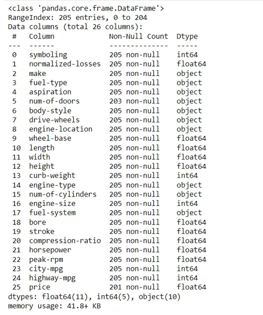
Since most of the sedan type cars are four doors,assuming that the both sedan cars have four doors
df2["num-of-doors"].replace(np.nan,"four", inplace=True)Finding the price using Random Forest Regressor
def encoder(datatype):
    t = LabelEncoder()
    for i in datatype:
        if datatype[i].dtype == "object":
            datatype[i] = t.fit_transform(datatype[i])
encoder(df2)
df2.head()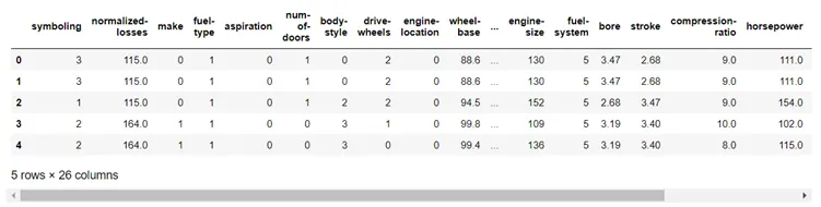
Scaling the dataset using MinMaxScaler
scaler=MinMaxScaler()
df2=pd.DataFrame(scaler.fit_transform(df2), columns=df2.columns)
Filtering the null value price rows
m_p = df2[df2['price'].isna()]
m_p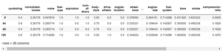
Removing the null value price rows
df2.dropna(subset=["price"], axis=0, inplace=True)
df2.reset_index(drop=True, inplace=True)
X = df2[df2.columns.drop(['price'])]
Y = df2['price']Splitting the dataset into test and train dataset
X_train, X_test, y_train, y_test = train_test_split(X,Y,test_size = 0.4, random_state=90)RF = RandomForestRegressor()
RF.fit(X_train,y_train)
Y_pred = RF.predict(X_test)
print(Y_pred)[0.31379177 0.6594963 0.10796481 0.11735713 0.04875676 0.05798669 0.05820913 0.01216151 0.04276103 0.68375552 0.10995941 0.10865076 0.19176779 0.1968224 0.05484062 0.07174619 0.11174979 0.10200611 0.19873467 0.02918673 0.39471302 0.07897696 0.0166176 0.71101758 0.12547043 0.02645003 0.04965667 0.01424656 0.20127352 0.21185691 0.77121841 0.34967876 0.29633186 0.11822191 0.11624448 0.27342845 0.10701058 0.10898499 0.38818927 0.12648789 0.03851398 0.07122859 0.05344943 0.12032372 0.24321906 0.2029075 0.29578919 0.38569659 0.03856958 0.0882759 0.65348592 0.11823461 0.09118341 0.36920783 0.26553299 0.01969192 0.12416944 0.28137195 0.2187091 0.12871589 0.14655156 0.11254245 0.03696763 0.21488605 0.12124721 0.35277568 0.03856958 0.20575791 0.5814463 0.23937863 0.23679708 0.28243955 0.11105895 0.12310892 0.2308587 0.08609776 0.23725336 0.15435281 0.0589864 0.59251502 0.11302741]
rf = RF.score(X_test,y_test)
print(rf)
0.9088761544334404
X1 = m_p[m_p.columns.drop(['price'])]Predicting the null-value price using random forest regressor
p = RF.predict(X1)
p
array([0.3214756 , 0.02299787, 0.0290564 , 0.7026245 ])
index = [200,201,202,203]
final_Array = []
c = 0
for l in index:
    if c<len(index):
        for j in p:
            final_Array.append(((l, j)))
            j+=1
            l+=1
            c+=1
data = pd.DataFrame(final_Array,columns=['index','price'])
data.head()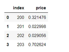
Reseting the index
X1.reset_index(drop=True, inplace=True)Joining the new price with the existing column
f = pd.concat([X1,data], axis=1)Setting index
f.set_index("index", inplace=True)
f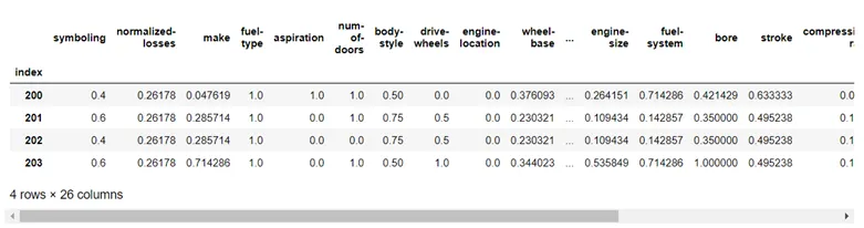
Combining the missing price dataset with df2
df2 = pd.concat([df2,f])df2.isnull().sum()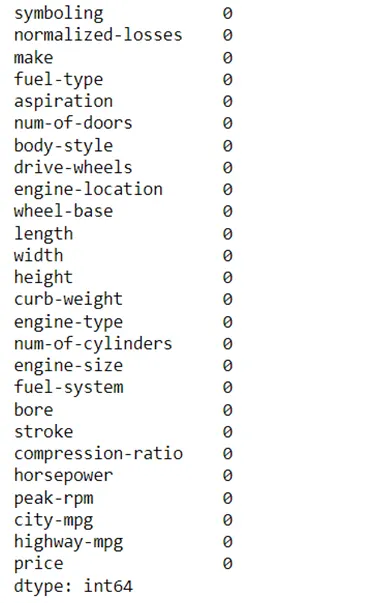
Plotting
plt.figure(figsize=(17,17))
sn.heatmap(data=df2.corr(),annot=True) # corretalional
plt.show()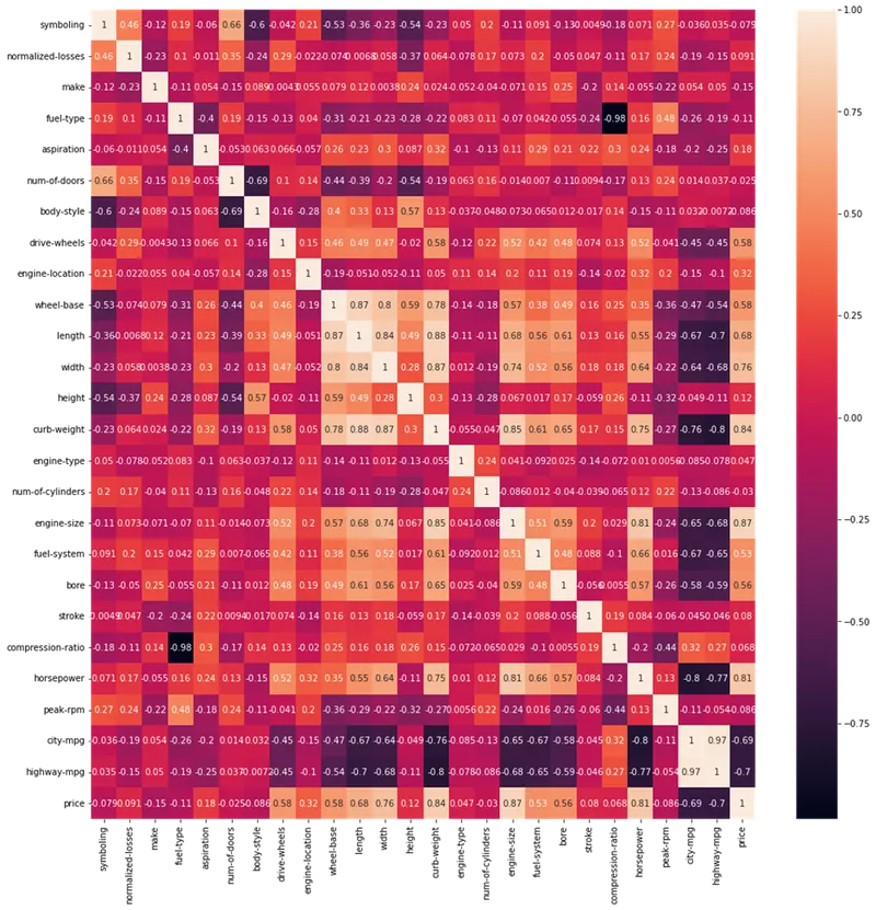
Performing PCA on the dataset
pca = PCA(n_components=3)
d_pca = pd.DataFrame(pca.fit_transform(df2),columns=['pc1','pc2','pc3'])
d_pca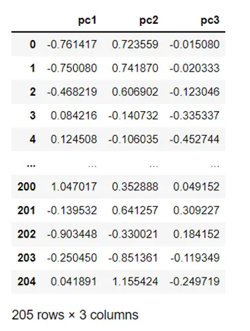
Implementing K-means to form class column
k_range=range(1,20)
sse=[]
for k in k_range:
    km=KMeans(n_clusters=k)
    km.fit(d_pca)
    sse.append(km.inertia_)
print(sse)
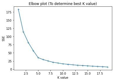
plt.plot(k_range, sse, '-+')
plt.xlabel('K value')
plt.ylabel('SSE')
plt.title('Elbow plot (To determine best K value)')
plt.show()
[182.734723477616, 114.60985735648904, 81.85969283379508, 56.99943652748497,
35.56070361085253, 29.54146540722608, 25.416432975144257, 21.352301605932805,
18.945979843146944, 16.58388640195327, 15.10720189601353, 13.602270043948335,
12.034749354562923, 11.489623078880674, 10.406934622932779, 9.415576706325817,
8.518812489508145, 7.893105020717661, 6.850086945580614]
Since elbow curve doesn't help to choose correct k values silhoutte score is used
for i in range(2,13):
    labels=cluster.KMeans(n_clusters=i).fit(d_pca).labels_
    print ("Silhouette score for k(clusters) = "+str(i)+" is "+str(metrics.silhouette_score(d_pca,labels,metric="euclidean")))
Silhouette score for k(clusters) = 2 is 0.40391133552680836 Silhouette score for k(clusters) = 3 is 0.4537742123882564 Silhouette score for k(clusters) = 4 is 0.4543734446698324 Silhouette score for k(clusters) = 5 is 0.5049600066530242 Silhouette score for k(clusters) = 6 is 0.5168513332218838 Silhouette score for k(clusters) = 7 is 0.47178574773325727 Silhouette score for k(clusters) = 8 is 0.4419244701735852 Silhouette score for k(clusters) = 9 is 0.4447355418092978 Silhouette score for k(clusters) = 10 is 0.4658308691009421 Silhouette score for k(clusters) = 11 is 0.4841685602067468 Silhouette score for k(clusters) = 12 is 0.4643317491683399
Based on silhouette score number of cluster is chosen as 6
kmeans = KMeans(n_clusters = 6)
y1 = pd.Series(kmeans.fit_predict(d_pca))
d_pca['class'] = y1
y1.value_counts()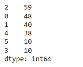
d_pca.head(10)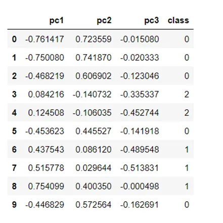
sn.pairplot(d_pca, hue="class")
plt.show()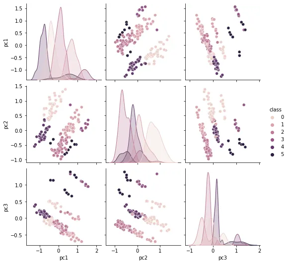
Using Classifier
1. KNN Classifier
X = d_pca[d_pca.columns.drop(['class'])]
y = d_pca['class']
X_train,X_test,y_train,y_test = train_test_split(X,y,test_size = 0.3, random_state =90) kn = KNeighborsClassifier(n_neighbors=6)
kn.fit(X_train,y_train)
y_pred = kn.predict(X_test)
y_predarray([2, 2, 2, 0, 5, 0, 4, 2, 0, 4, 1, 2, 2, 0, 1, 2, 4, 1, 4, 4, 2, 1,
0, 0, 2, 1, 2, 4, 2, 1, 4, 3, 2, 2, 2, 1, 0, 4, 0, 0, 0, 2, 1, 2,
2, 2, 2, 2, 4, 5, 1, 2, 5, 1, 2, 0, 4, 5, 4, 0, 2, 0])
knt = kn.score(X_test,y_test)
print(knt)
0.9838709677419355
cm = confusion_matrix(y_test, y_pred)
print(cm)
[[12 0 0 0 0 0] [ 0 10 0 0 0 0] [ 0 0 23 0 0 0] [ 0 0 0 1 0 0] [ 1 0 0 0 11 0] [ 0 0 0 0 0 4]]
print(classification_report(y_test, y_pred))precision recall f1-score support
0 0.92 1.00 0.96 12
1 1.00 1.00 1.00 10
2 1.00 1.00 1.00 23
3 1.00 1.00 1.00 1
4 1.00 0.92 0.96 12
5 1.00 1.00 1.00 4
accuracy 0.98 62
macro avg 0.99 0.99 0.99 62
weighted avg 0.99 0.98 0.98 62
plt.figure(figsize=(15,10))
categories = np.unique(y)
df_cm = pd.DataFrame(cm, index = [i for i in categories], columns = [i for i in categories])
sn.heatmap(df_cm,annot=True)
plt.xlabel("Predicted")
plt.ylabel("Actual")
plt.show()
2. Decision Tree
X = d_pca[d_pca.columns.drop(['class'])]
y = d_pca['class']
X_train,X_test,y_train,y_test = train_test_split(X,y,test_size = 0.3, random_state =90) DC = DecisionTreeClassifier()
DC.fit(X_train,y_train)
y_pred = DC.predict(X_test)
y_predarray([2, 2, 2, 4, 5, 0, 4, 2, 0, 4, 1, 2, 2, 0, 1, 2, 4, 1, 4, 4, 2, 1,
0, 0, 2, 1, 2, 4, 2, 1, 4, 3, 2, 2, 2, 1, 0, 4, 0, 0, 0, 2, 1, 2,
2, 2, 2, 2, 4, 5, 1, 2, 5, 1, 2, 0, 4, 5, 4, 0, 2, 0])
Dc = DC.score(X_test,y_test)
print(Dc)
1.0
print(classification_report(y_test, y_pred))precision recall f1-score support
0 1.00 1.00 1.00 12
1 1.00 1.00 1.00 10
2 1.00 1.00 1.00 23
3 1.00 1.00 1.00 1
4 1.00 1.00 1.00 12
5 1.00 1.00 1.00 4
accuracy 1.00 62
macro avg 1.00 1.00 1.00 62
weighted avg 1.00 1.00 1.00 62
cm = confusion_matrix(y_test, y_pred)
print(cm)
[[12 0 0 0 0 0] [ 0 10 0 0 0 0] [ 0 0 23 0 0 0] [ 0 0 0 1 0 0] [ 0 0 0 0 12 0] [ 0 0 0 0 0 4]]
plt.figure(figsize=(15,10))
categories = np.unique(y)
df_cm = pd.DataFrame(cm, index = [i for i in categories], columns = [i for i in categories])
sn.heatmap(df_cm,annot=True)
plt.xlabel("Predicted")
plt.ylabel("Actual")
plt.show()
3. Random Forest
X = d_pca[d_pca.columns.drop(['class'])]
y = d_pca['class']
X_train,X_test,y_train,y_test = train_test_split(X,y,test_size = 0.3, random_state = 90) Rtc = RandomForestClassifier()
Rtc.fit(X_train,y_train)
y_pred = Rtc.predict(X_test)
y_predarray([2, 2, 2, 4, 5, 0, 4, 2, 0, 4, 1, 2, 2, 0, 1, 2, 4, 1, 4, 4, 2, 1,
0, 0, 2, 1, 2, 4, 2, 1, 4, 3, 2, 2, 2, 1, 0, 4, 0, 0, 0, 2, 1, 2,
2, 2, 2, 2, 4, 5, 1, 2, 5, 1, 2, 0, 4, 5, 4, 0, 2, 0])
rc = Rtc.score(X_test,y_test)
print(rc)
1.0
print(classification_report(y_test, y_pred))precision recall f1-score support
0 1.00 1.00 1.00 12
1 1.00 1.00 1.00 10
2 1.00 1.00 1.00 23
3 1.00 1.00 1.00 1
4 1.00 1.00 1.00 12
5 1.00 1.00 1.00 4
accuracy 1.00 62
macro avg 1.00 1.00 1.00 62
weighted avg 1.00 1.00 1.00 62
cm = confusion_matrix(y_test, y_pred)
print(cm)
[[12 0 0 0 0 0] [ 0 10 0 0 0 0] [ 0 0 23 0 0 0] [ 0 0 0 1 0 0] [ 0 0 0 0 12 0] [ 0 0 0 0 0 4]]
plt.figure(figsize=(15,10))
categories = np.unique(y)
df_cm = pd.DataFrame(cm, index = [i for i in categories], columns = [i for i in categories])
sn.heatmap(df_cm,annot=True)
plt.xlabel("Predicted")
plt.ylabel("Actual")
plt.show()
4. SVM
X = d_pca[d_pca.columns.drop(['class'])]
y = d_pca['class']
X_train,X_test,y_train,y_test = train_test_split(X,y,test_size = 0.3, random_state =90) SVM = SVC()
SVM.fit(X_train,y_train)
y_pred = SVM.predict(X_test)
y_predarray([2, 2, 2, 0, 5, 0, 4, 2, 0, 4, 1, 2, 2, 0, 1, 2, 4, 1, 4, 4, 2, 1,
0, 0, 2, 1, 2, 4, 2, 1, 4, 3, 2, 2, 2, 1, 0, 4, 0, 0, 0, 2, 1, 2,
2, 2, 2, 2, 4, 5, 1, 2, 5, 1, 2, 0, 4, 5, 4, 0, 2, 0])
svm = SVM.score(X_test,y_test)
print(svm)
0.9838709677419355
print(classification_report(y_test, y_pred))precision recall f1-score support
0 0.92 1.00 0.96 12
1 1.00 1.00 1.00 10
2 1.00 1.00 1.00 23
3 1.00 1.00 1.00 1
4 1.00 0.92 0.96 12
5 1.00 1.00 1.00 4
accuracy 0.98 62
macro avg 0.99 0.99 0.99 62
weighted avg 0.99 0.98 0.98 62
cm = confusion_matrix(y_test, y_pred)
print(cm)
[[12 0 0 0 0 0] [ 0 10 0 0 0 0] [ 0 0 23 0 0 0] [ 0 0 0 1 0 0] [ 1 0 0 0 11 0] [ 0 0 0 0 0 4]]
plt.figure(figsize=(15,10))
categories = np.unique(y)
df_cm = pd.DataFrame(cm, index = [i for i in categories], columns = [i for i in categories])
sn.heatmap(df_cm,annot=True)
plt.xlabel("Predicted")
plt.ylabel("Actual")
plt.show()
Comparing the Classifier Models
df5 = pd.DataFrame([["KNN",knt],["Decision Tree",Dc],["Random Forest",rc],["SVM",svm]],columns=["models","accuracy"])
df5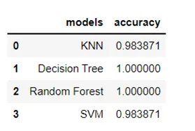
e = pd.DataFrame(df5.groupby('models')['accuracy'].mean())
e.plot.bar(title='models vs accuracy')
plt.xlabel("models")
plt.ylabel("accuracy")
plt.grid(linestyle='-.')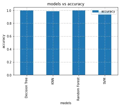
Observation
Random forest predicts the class of car with highest accuracy among the classifiers.