Implement and deploy CNN model in real-time using python on Fashion MNIST dataset

Introduction

Humans are a brilliant natural system which is having the great capability of viewing and observing multiple images in a short span of time, then consume and deduce from them without even realizing that how the actual process is completed. But this case is not at all similar with machines or systems.

Aim and Objectives

The main aim to plan and strategize a solution by understanding the basic idea of image processing for better understanding of the underlying concepts and then to get a vision of how to feed an image in such a manner that the machine or system can consume it to help and give a fruitful output.

Any image is a cumulative arrangement of dots called pixels and the pixels are arranged in a special order to represent an image. If the order structure or color of a pixel is modified in whatsoever way, the representation of image would be altered as well. So elaborate work has to be done on the implementation of CNN model.

About the Dataset

Here the dataset provided is based on certain fashion components, it is a dataset of images—consisting of a training set of 60,000 examples and a test set of 10,000 examples. Each example is a 28x28 grayscale image, associated with a label from 10 classes.

Data Description

1. Each image is 28 pixels in height and 28 pixels in width, for a total of 784 pixels in total.

2. Each pixel has a single pixel-value associated with it, indicating the lightness or darkness of that pixel, with higher numbers meaning darker. This pixel-value is an integer between 0 and 255.

3. The training and test data sets have 785 columns.

4. The first column consists of the class labels (see above), and represents the article of clothing.

5. The rest of the columns contain the pixel-values of the associated image.

To locate a pixel on the image, suppose that we have decomposed x as x = i * 28 + j, where i and j are integers between 0 and 27. The pixel is located on row i and column j of a 28 x 28 matrix. For example, pixel31 indicates the pixel that is in the fourth column from the left, and the second row from the top, as in a ascii-diagram.

Processing

Importing the libraries

import numpy as np
import pandas as pd
from tensorflow import keras 
from tensorflow.keras.utils import to_categorical

from tensorflow.keras.models import Sequential 
from tensorflow.keras.layers import Dense,Dropout,Activation,Flatten
from tensorflow.keras.layers import Conv2D,MaxPooling2D,BatchNormalization
from tensorflow.keras.losses import categorical_crossentropy
from sklearn.metrics import accuracy_score
from tensorflow.keras.regularizers import l2
from tensorflow.keras.preprocessing.image import ImageDataGenerator
from sklearn.metrics import classification_report,confusion_matrix
import matplotlib.pyplot as plt
import seaborn as sns

import warnings
warnings.filterwarnings('ignore')

Importing the dataset

train_data = pd.read_csv('fashion-mnist_train.csv')
train_data.shape

(60000, 785)

test_data = pd.read_csv('fashion-mnist_test.csv')
test_data.shape

(10000, 785)

train_data.head()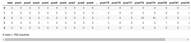

• The table above displays the first 5 rows of the data frame. Each row of this data frame contains information
  about an "image".
• The first column named label identifies the clothing item that is depicted in the image.
• The other 784 columns named pixel represent the image.

As we can see in above preview the mini dataset of 5 images is a matrix with 5 rows and 785 columns. Displaying it as matrix is not very informative as each cell is a pixel and as such is not human-readable. To better understand what each pixel represents, we need to convert it to a weighted form.

train_data.info()

<class 'pandas.core.frame.DataFrame'>
RangeIndex: 60000 entries, 0 to 59999
Columns: 785 entries, label to pixel784
dtypes: int64(785)
memory usage: 359.3 MB

• The dataframe statistics indicate that there are 60,000 rows and 785 features in the training dataset.
• Each row represents an image that will be used during model training.

Unique values in label column of training dataset

train_data['label'].unique()

array([2, 9, 6, 0, 3, 4, 5, 8, 7, 1], dtype=int64)

Counting number of images for each label class

train_data['label'].value_counts()

2    6000
9    6000
6    6000
0    6000
3    6000
4    6000
5    6000
8    6000
7    6000
1    6000
Name: label, dtype: int64

6,000 images associated with each label, it is balanced dataset

Separating independent and dependent variables for train and test data

train_x = train_data.drop(columns=['label'])
y_train = train_data['label']
test_x = test_data.drop(columns=['label'])
y_test = test_data['label']

train_x.shape, y_train.shape ,test_x.shape,y_test.shape

((60000, 784), (60000,), (10000, 784), (10000,))

• These are not in proper shape.
• For keras input shape size shoud be 4D.

Reshaping the data

x_train = train_x.values.reshape(train_x.shape[0],28,28,1) 
x_test = test_x.values.reshape(test_x.shape[0],28,28,1) 

print('x_train shape',x_train.shape)
print('x_test shape',x_test.shape)
print('y_train shape',y_train.shape)
print('y_test shape',y_test.shape)

x_train shape (60000, 28, 28, 1)
x_test shape (10000, 28, 28, 1)
y_train shape (60000,)
y_test shape (10000,)

Feature Scaling

• Each image is 28 pixels in height and 28 pixels in width, for a total of 784 pixels in total.
• The 784 pixelXXX column values in each row contain brightness information for each pixel in the 28x28 grayscale image.
• Each pixel has a single pixel-value associated with it, indicating the lightness or darkness of that pixel,
  with higher numbers meaning darker.
• This pixel-value is an integer between 0(black) and 255(white).Values in between represent different shades of gray.
• To normalize the values, we therefore need to divide each pixelXXX cell by 255.

Normalizing train & test data between 0 to 1

x_train = x_train/255
x_test = x_test/255

Visualizing the images

y_train.unique()

array([2, 9, 6, 0, 3, 4, 5, 8, 7, 1], dtype=int64)

Numeric labels are not that meaningful in a visualization, we'll map them to a textual representation
0 => T-shirt/top,1 => Trouser,2 => Pullover,3 => Dress,4 => Coat,5 => Sandal,6 => Shirt,7 => Sneaker,8 => Bag,9 => Ankle boot

class_labels = ['T shirt/top','Trouser','Pullover','Dress','Coat','Sandal','Shirt','Sneaker','Bag','Ankle boot']

Set figure size

plt.figure(figsize = (10,10))

Showing randomly 20 images from training dsataset

j=1
for i in np.random.randint(0,6000,20):
    plt.subplot(6,5,j)
    j+=1
    plt.xticks([])
    plt.yticks([])
    plt.imshow(x_train[i],cmap = plt.cm.binary)
    plt.title('{}/{}'.format(class_labels[y_train[i]],y_train[i]))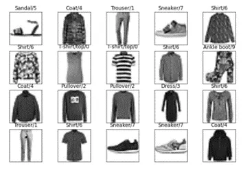

Train-test split dataset

from sklearn.model_selection import train_test_split
x_train,x_val,y_train,y_val = train_test_split(x_train,y_train,test_size = 0.2,random_state=42)

x_train.shape , y_train.shape

((48000, 28, 28, 1), (48000,))

x_val.shape , y_val.shape

((12000, 28, 28, 1), (12000,))

Convolutional Neural Network - Model Building

model = keras.models.Sequential([
                                keras.layers.Conv2D(filters = 32,kernel_size = 3,padding = 'valid',activation = 'relu',input_shape = [28,28,1]),
                                keras.layers.MaxPooling2D(pool_size = (2,2)),
                                keras.layers.Conv2D(filters = 64,kernel_size = 3,padding = 'same',activation = 'relu'),
                                keras.layers.MaxPooling2D(pool_size = (2,2)),
                                keras.layers.Flatten(),
                                keras.layers.Dense(units=256, activation='relu'),
                                keras.layers.Dropout(0.5),                  
                                keras.layers.Dense(units = 128,activation = 'relu'),
                                keras.layers.Dropout(0.10),
                                keras.layers.Dense(units = 10,activation = 'softmax')])

Model summary

model.summary()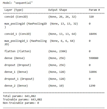

Model compile

model.compile(optimizer = 'adam',loss = 'sparse_categorical_crossentropy',metrics = ['accuracy'])

Train

history = model.fit(x_train,y_train,epochs = 15,batch_size = 512,verbose = 1 , validation_data = (x_val,y_val))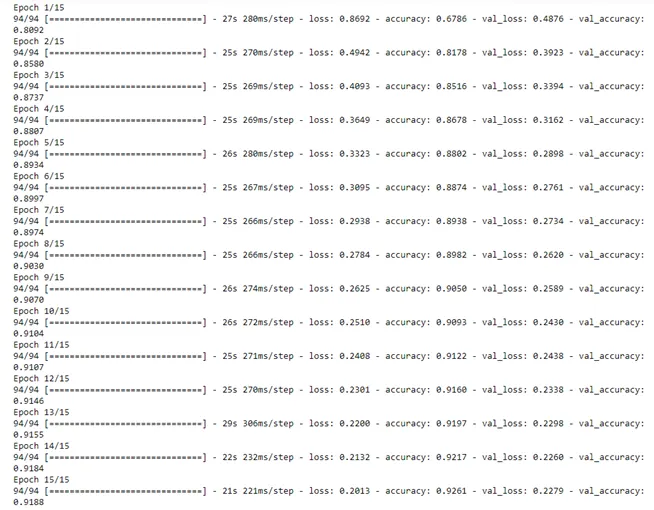

List of all the data in history

print(history.history.keys())

dict_keys(['loss', 'accuracy', 'val_loss', 'val_accuracy'])

Plotting accuracy and loss of the model

def plot_training_hist(history):
    '''Function to plot history for accuracy and loss'''
    
    fig, ax = plt.subplots(1, 2, figsize=(10,4))
    
    # first plot
    ax[0].plot(history.history['accuracy'])
    ax[0].plot(history.history['val_accuracy'])
    ax[0].set_title('Model Accuracy')
    ax[0].set_xlabel('epoch')
    ax[0].set_ylabel('accuracy')
    ax[0].legend(['train', 'validation'], loc='best')
    
    # second plot
    ax[1].plot(history.history['loss'])
    ax[1].plot(history.history['val_loss'])
    ax[1].set_title('Model Loss')
    ax[1].set_xlabel('epoch')
    ax[1].set_ylabel('loss')
    ax[1].legend(['train', 'validation'], loc='best')
    
plot_training_hist(history)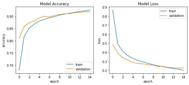

Test Model

np.argmax(model.predict(np.expand_dims(x_test[0],axis = 0)).round(2)) 
#test on single test image(predicted label)

0

y_test[0] #actual label of above image

y_pred = model.predict(x_test).round(2)
y_pred

array([[1.  , 0.  , 0.  , ..., 0.  , 0.  , 0.  ],
       [0.  , 1.  , 0.  , ..., 0.  , 0.  , 0.  ],
       [0.01, 0.  , 0.87, ..., 0.  , 0.  , 0.  ],
       ...,
       [0.  , 0.  , 0.  , ..., 0.  , 1.  , 0.  ],
       [0.  , 0.  , 0.  , ..., 0.  , 1.  , 0.  ],
       [0.  , 1.  , 0.  , ..., 0.  , 0.  , 0.  ]], dtype=float32)

Model evaluation

model.evaluate(x_test,y_test)

[0.2102140635251999, 0.9229000210762024]

Visualize output

plt.figure(figsize = (16,30))

Comparing randomly actual and predicted labels from test data

j=1
for i in np.random.randint(0,1000,10):
    plt.subplot(10,5,j);j+=1
    plt.xticks([])
    plt.yticks([])
    plt.imshow(x_test[i].reshape(28,28),cmap = 'Greys')
    plt.title('Actual = {} / {}  npredicted = {} / {}'.format(class_labels[y_test[i]],y_test[i],class_labels[np.argmax(y_pred[i])],np.argmax(y_pred[i])))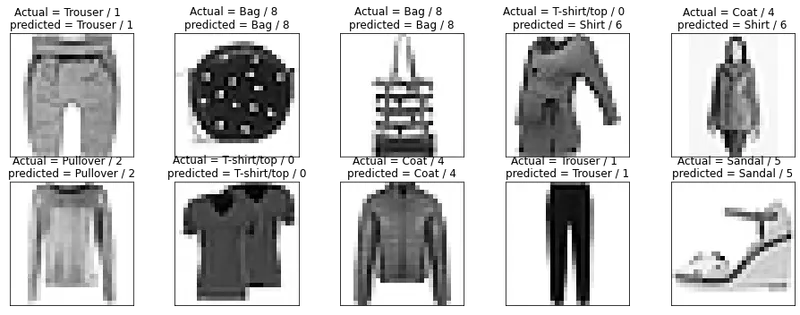

Confusion Matrix

from sklearn.metrics import confusion_matrix

y_predicted_labels = [np.argmax(label) for label in y_pred]
cm = confusion_matrix(y_test,y_predicted_labels)

print('confusion_matrix:n',cm)

confusion_matrix:
 [[900   0  16  11   0   0  68   0   5   0]
 [  2 983   1  12   0   1   1   0   0   0]
 [ 12   0 881  12  47   0  44   0   4   0]
 [ 13   3   3 949  17   0  15   0   0   0]
 [  1   0  30  24 899   0  46   0   0   0]
 [  0   0   0   0   0 980   0  13   1   6]
 [133   2  46  28  63   0 719   0   9   0]
 [  0   0   0   0   0   5   0 961   0  34]
 [  3   1   2   0   2   1   2   2 986   1]
 [  0   0   0   0   0   1   0  27   0 972]]

Plotting the confusion matrix

plt.figure(figsize=(10,7))
sns.heatmap(cm,annot = True,fmt = 'd',xticklabels=class_labels, yticklabels=class_labels)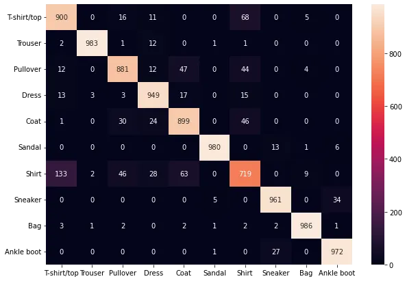

Classification report

cl_report = classification_report(y_test,y_predicted_labels , target_names = class_labels)
print(cl_report)

              precision    recall  f1-score   support

 T-shirt/top       0.85      0.90      0.87      1000
     Trouser       0.99      0.98      0.99      1000
    Pullover       0.90      0.88      0.89      1000
       Dress       0.92      0.95      0.93      1000
        Coat       0.87      0.90      0.89      1000
      Sandal       0.99      0.98      0.99      1000
       Shirt       0.80      0.72      0.76      1000
     Sneaker       0.96      0.96      0.96      1000
         Bag       0.98      0.99      0.98      1000
  Ankle boot       0.96      0.97      0.97      1000

    accuracy                           0.92     10000
   macro avg       0.92      0.92      0.92     10000
weighted avg       0.92      0.92      0.92     10000

We can say from above report:

• Trouser, sandal, bag, ankle boot model performance is very good.
  
• Shirt model performance is not very good comparatively