Steady Vs Unsteady flow over a cylinder

OBJECTIVE: To simulate the flow over a cylinder using unsteady and steady state solvers.

INTRODUCTION: In fluid dynamics, vortex shedding is an oscillating flow that takes place when a fluid such as air or water flows past a bluff (as opposed to streamlined) body at certain velocities, depending on the size and shape of the body. In this flow, vortices are created at the back of the body and detach periodically from either side of the body forming a Von Karman vortex street which is responsible for the unsteady separation of the flow of a fluid around blunt bodies. It is named after the engineer and fluid dynamicist Theodore von karman. The fluid flow past the object creates alternating low-pressure vortices on the downstream side of the object. The object will tend to move toward the low-pressure zone.

A vortex street will form only at a certain range of flow velocities, specified by a range of Reynolds numbers(Re), typically above a limiting Re value of about 90. The Reynolds number for a flow is a measure of the ratio of inertial to viscous forces in the flow of a fluid around a body or in a channel.

• = the free stream flow speed
• = a characteristic length parameter of the body or channel
• = the free stream kinematic viscosity

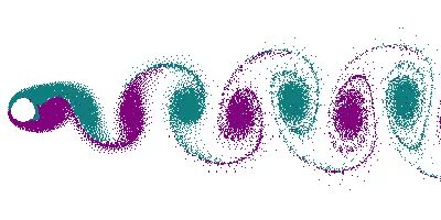
Animation of vortex street created by a cylindrical object; the flow on opposite sides of the object is given different colors, showing that the vortices are shed from alternating sides of the object.

PROCEDURE:

1. Geometry:

• First the cylinder boundary is to be drawn in the spaceclaim and its dimensions are as below:

• Now the inside circle is to be deleted to carry out the simulation.

2.Mesh:

• Now in the mesh mode we set the mesh size and give inflation layers to the cylinder.
• The mesh size given is 0.25m and inflation layers are 6 no.s and with first layer thickness and first layer height of 0.005.

3. Solving:

• Now launch the setup and set the conditions as below and select laminar as the model.

Here, Area = Height*Width = `2m^2`

Height = 2m

Width = 1m because analysis is 2D

For all 2D problems Depth =1m

Length = 2m (because here length means flow length along the direction of flow which is the diameter = 2m)

Steady State Simulation:

PLOTS: In both i.e. steady and unsteady state simulations, following plots are to be shown:

1. Residual plot - This plot helps us in knowing at what point convergence is achieved.

2. Monitor point velocity plot - A monitor point is placed at a distance of 8m from the cylinder inorder to calclate the velocity at that point.

3. Drag coefficient plot - To calculate the drag coefficient.

4. Lift coefficient plot - To calculate the lift coefficient.

5. Velocity contour plot - To see the velocity changes in the flow over the cylinder.

Case-1: For Re=10 where viscosity=0.02 and velocity=0.1m/s

Residual plot: Residual plot helps us in knowing the convergence point of the simulation.

Monitor point velocity:

Drag coefficient:

Lift coefficient:

velocity contour:

Case-2: For Re=100 where viscosity=0.02 and velocity=1m/s

Residual plot:

Monitor velocity:

Drag coefficient:

Lift coefficient:

Velocity contour:

Case-3: For Re=1000 where viscosity=0.02 and velocity=10m/s

Residual plot:

Monitor point velocity:

Drag coefficient:

Lift coefficient:

Velocity Contour:

Case-4: For Re=10000 where viscosity=0.02 and velocity=100m/s

Residual plot:

Monitor point velocity:

Drag Coefficient:

Lift Coefficient:

Velocity contour:

Case-5: For Re=100000 where viscosity=0.00002 and velocity=1m/s

Residual Plot:

Monitor velocity plot:

Drag coefficient:

Lift coefficient:

Velocity contour:

Summary Table: Cd and Cl values for the respective reynolds number carried out for the steady state

Effect of Reynolds Number on Drag Coefficient(Cd):

Here we see that as reynolds number increases, drag coefficient decreases till Re = 1000 but at Re = 10000 we see a slight increase in drag coefficient and again for Re = 100000 the drag oefficient value decreases.

Unsteady State Simulation:

For Re=100 where viscosity=0.02 and velocity=1m/s.

Time step size = 0.1

Residual plot:

Monitor point velocity:

Drag coefficient:

Lift coefficient:

Cd and Cl values for transient condition:

Cd	Cl
1.33	0.25

Velocity contour:

Strouhal Number:

The Strouhal Number is a dimensionless value useful for analyzing oscillating unsteady fluid flow dynamics problems.

Strouhal number cannot be calculated for the steady state as there is no time parameter which is required in frequency calculation and can only be calculated for unsteady state condition.

The Strouhal Number can be expressed as

`St=(omega*L)/v`

where St = Strouhal Number

`omega`= oscillation frequency

L = characteristic frequency

v = flow velocity

The Strouhal Number can be important when analyzing unsteady, oscillating flow problems. The Strouhal Number represents a measure of the ratio of the inertial forces due to the unsteadiness of the flow or local acceleration to the inertial forces due to changes in velocity from one point to an other in the flow field.

`omega =`No.of peaks/Flow time = 3/20 = 1.5Hz

`St=(1.5*2)/1=0.3`

4.Conclusion:

• Steady and unsteady state simulations were carried out for the flow over cylinder and residual,monitor point velocity,drag and lift values were computed and plotted.
• Different reynolds number were introduced to see the vortex shedding phenomena behind the cylinder.
• Strouhal number was calculated for the transient condition.