Project 2 - Rankine cycle Simulator
RANKINE CYCLE
The Rankine cycle is one of the most common operating cycles for all power plants, where the working fluid is continuously changing its phase from liquid to vapor and vice versa. The cycle generates power by converting the pressure energy of steam into mechanical energy through the steam turbine (which can be further converted to other energy as desired). The four major components of a Rankine cycle are the pump, boiler, turbine, and condenser.
PUMP: In the cycle, the pump compresses the fluid (water) fed and sends it to the boiler,( as we are taking into consideration an ideal cycle the temperature remains constant during the compression.)
BOILER: The compressed fluid (water) from the pump is heated until it gets evaporated and send to the turbine, (there is an increase in temperature and pressure along with phase change.)
TURBINE: In the turbine, the high pressure and temperature gas (steam) are sent from the boiler, which further expands and rotates the turbine generating mechanical energy after that the gas is sent to the condenser.
CONDENSER: The gas (steam) received from the turbine is cooled by heat exchange and the phase changes back to fluid (water) which is again fed to the pump and the cycle goes on.
The processes involved in the components of the Rankine cycle are.
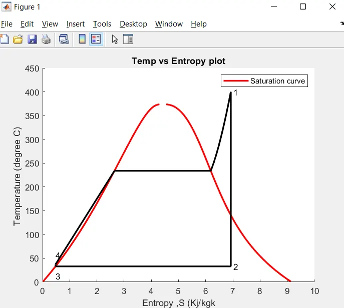
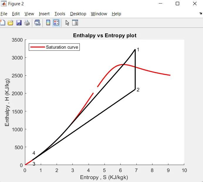
1-2: Isentropic expansion in turbine.
2-3: Constant pressure heat rejection in the condenser.
3-4: Isentropic compression in the pump.
4-1: Constant pressure heat addition in the boiler.
The cycle we are referring to is an ideal Rankine cycle so neglecting losses
In the 1-2 process (Isentropic expansion) the vapor expands through the turbine causing it to move, which generates the power . The overall expansion in the ideal cycle is adiabatic and reversible so it is referred isentropic. the drop in the temperature and pressure may cause some condensation.
2-3 process(Constant pressure heat rejection), the semi-liquid vapor from the turbine is passed to the condenser where the heat rejection occurs from the vapor as it is supplied to the condensing medium. The temperature drop results in the changing of vapor to fluid.
3-4 process(Isentropic compression), the fluid from the condenser is later supplied to the pump where it is compressed isentropically thus increasing its pressure so that it can be fed to the boiler.
4-1 process(Constant pressure heat addition), the pressure increased fluid is fed to the boiler where the temperature is increased as the heat is added to the fluid .which causes the fluid to change to vapor .thus the process occurs in a loop generating power.
The most used fluid for the cycle is water as its properties are favorable and its abundance in nature.
MATLAB PROGRAM FOR RANKINE CYCLE SIMULATOR
clear all
close all
clc

%Presentation
disp('               RANKINE CYCLE STIMULATOR         ' );
disp(' 1-2 is Isentropic Expansion in the Turbine ');
disp(' 2-3 is Constant Pressure Heat Rejection by Condenser ' ) ;
disp(' 3-4 is Isentropic Compression in the Pump');
disp(' 4-1 is Constant Pressure Heat Addition by the Boiler ');
fprintf('\n')
 %Input data
T1 = input(" Enter the temperature at turbine inlet(in degree.c) =");
p1 = input(" Enter the pressure at Turbine inlet(in bar) =");
p2 = input(" Enter the temperature at condenser (in bar) =");

% Extracting data
% State 1
h1 = XSteam('h_pT', p1, T1);
s1 = XSteam('s_pT', p1, T1);
% State 2
s2 = s1;
sf2= XSteam('sL_p', p2);
sg2 = XSteam('sV_p', p2);
x2 = (s2-sf2)/(sg2-sf2);
hf2 = XSteam('hL_p', p2);
hg2 = XSteam('hV_p', p2);
h2 = hf2 + (x2*(hg2-hf2));
% State 3
p3 = p2;
s3= XSteam('sL_p', p3);
h3 = XSteam('hL_p', p3);
% State 4
s4 = s3;
p4 = p1;

% Work done (turbine)
Wt = h1 - h2;

% Work done (pump)
v3 = XSteam('vL_p', p3);
Wp = v3*(p4 - p3)*100;
h4 = h3 + Wp;

%net work
Wnet = Wt - Wp;

%Heat taken in the system
Qin = h1 - h4;

%Heat given out by the system
Qout = h2 - h3;

%Thermal efficiency
T_eff = (Wnet/Qin)*100;

%Specific Steam Consumption = (Mass flow rate / Net work done)
SSC = (3600/Wnet);

%Calculating temperatures at the state points
T3 = XSteam('Tsat_p', p3);
T2 = T3;
Cp4 = XSteam('Cp_ps', p4, s4);
Cv4 = XSteam('Cv_ps', p4, s4);
k = Cp4/Cv4;
T4 = T3/((p3/p4)^((k-1)/k));

%Calculating temperature, entropy and enthalpy at the vapour and liquid
T6 = XSteam('Tsat_p', p1);
s5 = XSteam('sL_p', p1);
s6 = XSteam('sV_p', p1);
h5 = XSteam('hL_p', p1);
h6 = XSteam('hV_p', p1);
T5 = T6;

%Plotting the saturation curve
T = linspace(1,500,1000);
for i = 1:length(T)

sf(i) = XSteam('sL_T', T(i));
sg(i) = XSteam('sV_T', T(i));
hf(i) = XSteam('hL_T', T(i));
hg(i) = XSteam('hV_T', T(i));
end

%Plotting T-s diagram
figure(1)
hold on
plot(sf, T ,'color', 'r','linewidth',2)
plot(sg , T ,'color', 'r','linewidth',2)
plot([s1 s2], [T1 T2],'color', 'k', 'linewidth', 2)
plot([s2 s3], [T2 T3] ,'color','k', 'linewidth', 2)
plot([s3 s4], [T3 T4] ,'color', 'k', 'linewidth', 2)
plot([s4 s5], [T4 T5] ,'color', 'k', 'linewidth', 2)
plot([s5 s6], [T5 T6] ,'color', 'k', 'linewidth', 2)
sc1 = linspace(s6, s1 , 1000);
for l = 1:length(sc1)
 Tc1(l) = XSteam('T_ps', p1, sc1(l));
end
plot(sc1, Tc1,'color', 'k', 'linewidth', 2)
text(s1+0.1, T1, '1')
text(s2+0.1, T2, '2')
text(s3, T3-20, '3')
text(s4, T4+20, '4')
title('Temp vs Entropy plot')
xlabel('Entropy ,S (Kj/kgk')
ylabel('Temperature (degree C) ')
legend('Saturation curve')

%Plotting h-s diagram
figure(2)
hold on
plot(sf, hf,'color', 'r', 'linewidth', 2)
plot(sg, hg,'color', 'r',  'linewidth', 2)
plot([s1 s2], [h1 h2],'color', 'k', 'linewidth', 2)
plot([s2 s3], [h2 h3],'color', 'k', 'linewidth', 2)
plot([s3 s4], [h3 h4],'color', 'k', 'linewidth', 2)
hc = linspace(h4, h5, 100);
for k = 1:length(hc)
sch(k) = XSteam('s_ph', p1, hc(k));
end
plot(sch,hc,'color', 'k', 'linewidth', 2)
plot([s5 s6], [h5 h6],'color', 'k', 'linewidth', 2)
for m = 1:length(sc1)
hc1(m) = XSteam('h_ps', p1, sc1(m));
end
plot(sc1, hc1,'color', 'k', 'linewidth', 2)
text(s1+0.1, h1, '1')
text(s2+0.1, h2, '2')
text(s3, h3-100, '3')
text(s4, h4 +200, '4')
title('Enthalpy vs Entropy plot')
xlabel('Entropy , S (KJ/kgk) ')
ylabel('Enthalpy , H (KJ/kg)')
legend('Saturation curve','location','northwest')

% Displaying Results
fprintf('\n')
disp('                       RESULTS             ');
fprintf(' At State Point 1:\t\t\t\t\t');
fprintf('At State Point 2:\n');
fprintf(' p1 is : %7f bar\t\t\t\t', p1);
fprintf(' p2 is : %7f bar\n', p2);
fprintf(' T1 is : %7f C \t\t\t\t', T1);
fprintf(' T2 is : %7f C\n', T2);
fprintf(' h1 is : %7f KJ/kg\t\t\t', h1);
fprintf(' h2 is : %7f kJ/kg\n', h2);
fprintf(' s1 is : %7f KJ/kgK\t\t\t', s1);
fprintf(' s2 is : %7f kJ/kgK\n', s2);
fprintf(' x2 is : %7f\n', x2);
fprintf('\n')
fprintf(' At State Point 3:\t\t\t\t\t');
fprintf('At State Point 4:\n');
fprintf(' p3 is : %7f bar\t\t\t\t', p3);
fprintf(' p4 is : %7f bar\n', p4);
fprintf(' T3 is : %7f K\t\t\t\t', T3);
fprintf(' T4 is : %7f K\n', T4);
fprintf(' h3 is : %7f kJ/kg\t\t\t', h3);
fprintf(' h4 is : %7f KJ/kg\n', h4);
fprintf(' s3 is : %7f kJ/kgK\t\t\t', s3);
fprintf(' s4 is : %7f kJ/kgK\n\n', s4);
fprintf(' Wt is         : %7f kJ/kg\n', Wt);
fprintf(' Wp is         : %7f kJ/kg\n', Wp);
fprintf(' Wnet is       : %7f kJ/kg\n', Wnet);
fprintf(' Efficiency is : %7f Percent\n ', T_eff);
fprintf('S.S.C is      : %7f kJ/kWh\n', SSC);
clear all, close all, clc is used to close the graphical tabs, clear the data stored in the workspace, and clear the command window.
STEP 1: Presentation, the title, and the process of the Rankine cycle can be displayed with the help of 'disp' command by entering the text that is to be displayed in the command enclosing in an inverted comma.
STEP 2: Input data, for the calculation of overall state points of the Rankine cycle, some parameters are to be provided such as inlet and outlet temperature pressures. which can be given from the user end with the help of the 'input' command in which the required parameter to be entered can be asked in text and by assigning it to a variable that can be stored and used when it is called.
STEP 3: Extracting steam and water properties, with the help of XSteam file we can extract the steam and water properties of enthalpy, entropy at a specific pressure and temperatures for sat liquid, sat vapor conditions, etc. The Xsteam can be accessed by giving the temperature and pressure and what data is to be extracted enthalpy (h), entropy(s) along with at sat liquid and vapor ie. h1 = XSteam('h_pT', p1, T1); with this, all the defining variables can be extracted for the state points.
STEP 4: Thermodynamic relations, by using the thermodynamic relations we can further find the state point and with respect to it we can again extract their data from Xsteam.
STEP 5: Calculating work, with the help of thermodynamic relation and formula we can calculate the net work , work done by the turbine, work done to run the pump, Heat in, and heat out a.Efficiency and Specific steam consumption (s.s.c) of the Rankine cycle can be calculated as we have the other parameters.
STEP 6: Plotting, with the help of the extracted data and the parameters, using a 'for' loop and providing the parameter range we can plot the temperature, pressure, entropy, and enthalpy with respect to each other. t-s,h-s, and saturation curve can be plotted. we can position the legend by giving the direction within the command.
STEP 7: Result, with 'disp' and 'fprintf' commands we can display and print the calculated and extracted state point. by providing the float length we can limit the unit digit ie '%8f'.'\n' and '\t' is used to get to next line and to give space in between the text. Thus we can format the displaying output.
OUTPUT
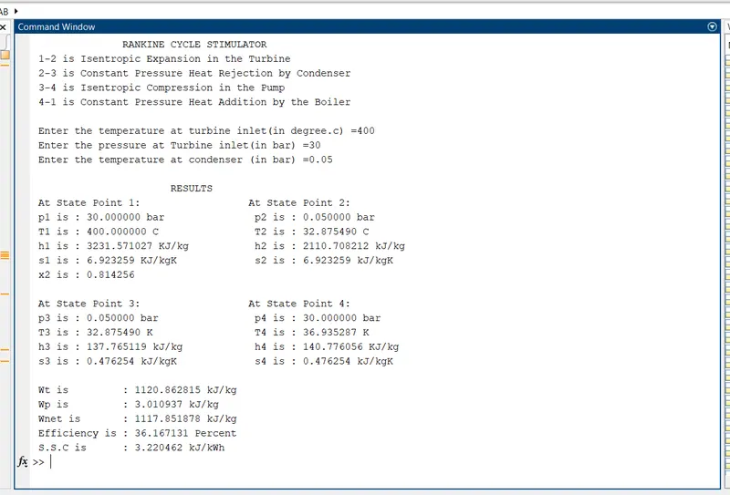
Input given
Enter the temperature at turbine inlet(in degree.c) =400
Enter the pressure at Turbine inlet(in bar) =30
Enter the temperature at condenser (in bar) =0.05
T-S diagram
H-S diagram
Command window
Conclusion
we have created a Rankin cycle simulator that takes input from the user and calculates the work and efficiency. which takes the steam data from provided Xsteam file.
Reference
https://www.thermal-engineering.org/what-is-rankine-cycle-steam-turbine-cycle-definition/
https://averyrh2.wixsite.com/website/projects
https://www.mathworks.com/help/matlab/matlab_prog/formatting-strings.html