Week 4.1 - Genetic Algorithm
Genetic Algorithm
A genetic algorithm works basically on the process of natural selection which is “survival of the fittest” among individuals of consecutive generations for solving a problem. Each generation consists of a population of individuals and each individual represents a point in search space and a possible solution. Each individual is represented as a string of character /integer /float /bits. This string is analogous to the Chromosome. The algorithm begins by creating a random initial population of individual selection and it keeps on modifying the population repeatedly creating a sequence of the new populations, the algorithm uses the individuals in the current generation to create the next population the genetic algorithm selects individuals at random from the current population to be parents and use them to produce the children for the next generation over successive generations the population evolves towards an optimum solution
The syntax for 'ga'
'ga' in Matlab is used to find the minima of function using a genetic algorithm
syntax is as follow
x=ga(@fun,nvars,A,B, Aeq, Beq,lb,ub,nonlcon,intcon,options)
where,
fun =Objective function.
nvars = number of variables.
A , B = Linear inequality constraints.
Aeq , Beq = Linear equality constraints.
if there are no linear equality and inequality,then A,B,Aeq,Beq are set to '[]'.
lb, ub = Lower and Upper bound that is the region in which Ga will search for the result.
nonlcon = non-Linear inequalities.
intcon = Integer constrained.
options= optimization options.
Program to optimize the stalagmite function and find the global maxima of the function
defining the stalagmite function
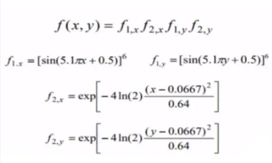
stalagmite function helps to generate local maxima and minima it is a three-dimensional function having peaks and valleys.
it is given as:
with the help of the stalagmite function, we can make the MatLab function code
function[f] = stalagmite(input_vector)
x = input_vector(1);
y = input_vector(2);
f1_x = (sin(5.1*pi.*x+0.5))^6;
f1_y = (sin(5.1*pi.*y+0.5))^6;
f2_x = exp(-4*log(2).*((x - 0.0667)^2/0.64));
f2_y = exp(-4*log(2).*((y - 0.0667)^2/0.64));
 f = -(f1_x.*f2_x.*f1_y.*f2_y);
 end
the negative sign in the function will invert the plotting which means we can get the maxima instead of minima.
Next GA code for stalagmite function
clear all
close all
clc

%defining the search space
x = linspace(0,0.6,150);
y = linspace(0,0.6,150);
rng('default')
no_case = 50
%creating 2D mesh
[xx yy] = meshgrid(x ,y);

%Evaluating the stalagmite function
for i = 1:length(xx)
  for j = 1:length (yy)
    input_vector(1)=xx(i,j);
    input_vector(2)=yy(i,j);
    f(i,j) = stalagmite(input_vector);

  end
end

 %study one with unbounded inputs
 tic
for i=1:no_case
[inputs, fopt(i) ]= ga(@stalagmite, 2);
xopt(i)=inputs (1) ;
yopt(i)=inputs (2);
end
study1_time = toc
figure(1)
subplot (2,1,1)
surfc (xx,yy, -f)
hold on
shading interp
plot3(xopt, yopt, -fopt, 'marker', 'o', 'markersize' ,5, 'markerfacecolor', 'r')
title( 'study 1 with unbounded inputs ')
xlabel('X-axis ')
ylabel('Y-axis ')
subplot (2,1,2)
plot (-fopt)
xlabel('Iterations')
ylabel('Function Maxima')

%study two with bounded input

 tic
for i=1:no_case
[inputs, fopt(i) ]= ga (@stalagmite, 2, [], [],[],[], [0;0], [1;1]);
xopt(i)=inputs (1) ;
yopt(i)=inputs (2);
end
study2_time = toc
figure(2)
subplot (2,1,1)
surfc (xx,yy, -f)
hold on
shading interp
plot3(xopt, yopt, -fopt, 'marker', 'o', 'markersize' ,5, 'markerfacecolor', 'r')
title('study 2 with bounded inputs')
xlabel('X-axis ')
ylabel('Y-axis ')
subplot (2,1,2)
plot (-fopt)
xlabel('Iterations')
ylabel('Function Maxima')

%study three with increased iteration
opt = optimoptions('ga');
opt = optimoptions(opt,'populationsize',300);
tic
for i=1:no_case
[inputs, fopt(i) ]= ga (@stalagmite, 2, [],[],[],[], [0;0], [1;1],[],[],opt);
xopt(i)=inputs (1) ;
yopt(i)=inputs (2);
end
study3_time = toc
figure(3)
subplot (2,1,1)
surfc (xx,yy, -f)
hold on
shading interp
plot3(xopt, yopt, -fopt, 'marker', 'o', 'markersize' ,5, 'markerfacecolor', 'r')
title( 'study 3 with increased iteration ')
xlabel('X-axis ')
ylabel('Y-axis ')
subplot (2,1,2)
plot (-fopt)
xlabel('Iterations')
ylabel('Function Maxima')
clear all, close all, clc is used to close the graphical tabs, clear the data stored in the workspace, and clear the command window.
Step 1: Define the x and y array which we can do with the help of 'linspace' , creating 150 equal intervals ie linspace (0,0.6,150) for both .'rng('default')' is used to control the random number generation keeping it default every time iterating or executing the code so that there is no much change in the output as the GA is random processing for optimum solution there may be a small variation in the output.
Step 2: To make a 2D mesh of x and y which can be created with the help of "meshgrid" command and the number of iterations to be performed can be defined with the help of the 'no_case' variable assigning value 50
Step 3: loop creation for the evaluation of stalagmite function, which can be done with a 'for' loop where 'i' is initialized, and for every value of 'i' another 'for' loop is used to initialize 'j' the input values of 'xx' and 'yy' are assigned and the stalagmite function for these input vector is defined .with this the basic structure is generated and we can also plot it separately.
Step 4:optimization using three cases, study one which can be done using 'for' loop where we use 'ga' syntax to give values for the input and optimum max value. In the 'ga' syntax stalagmite function is called and the number of variables 'nvar' is 2 to obtain the time required 'tic' and 'toc' command is used.
Step 5:Study one plotting, which can be done with 'surfc' command for 'xx,yy, and function output'.To obtain a smooth and clear plot 'shadinginterp' command can be used. the 'subplot(2,1,1)' is used to plot multiple plots on the same figure which also divides the figure into a grid of 2x1 and axes to be placed at 1 and the 'plot3' command plots the 3D points at 'xopt','yopt', and the optimum value function with 'o' shaped and red color.the labels and title can be also given with the help of 'xlabel' and 'title' command and in the same figure value of the optimum function, 'fopt' are plotted for 50 iterations.
Step 6: study two and its plotting, as from the study one the results generated will be different each time when we will run the program. so to get the same value each time we need to restrict the program within specific bounds ie upper and lower bounds, and by adding the lower limits and upper limit [0;0] and [1;1] into the 'ga' syntax of study one our study two code is ready the plotting code will be same as study one only the title can be changed to study two.
Step 7: Study three and plotting, it is observed that the results in study two are not the same every time the program terminates. A solution to this is by increasing the iteration so in study three we will increase the iteration to 300 and do so the syntax 'option=optimoptions('solvername','name', 'value')' is used which returns the named parameter 'populations' with alternate value '300'.the code of study three will be the same as study two only 'options' is added to the 'ga' syntax along with nonlinear equalities and inequalities which will be '[]' as they are not there. Rest all the code is the same for plotting also apart from 'title'.
OUTPUT.
Study one with unbounded inputs
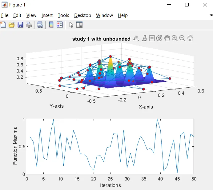
In the above plot, we can see that random sampling of the genetic algorithm generates a new optimum value for the function every time the code runs . the red dots show the values of x and y coordinates varying on each time iteration run.
Study two with bounded inputs.
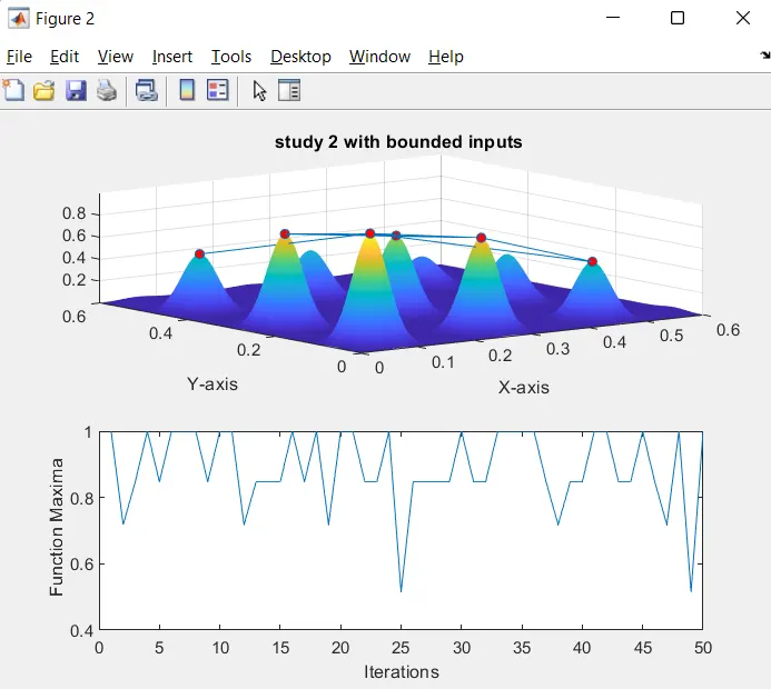
The above plots show the convergence of x and y values. the number of red dots has decreased as compared to study one. This is because of the bounds given upper and lower to the function
Study three with increased iteration
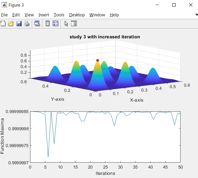
In this plot, the iteration was increased to 300 to converge and find the global maxima. Here we can see there is only one red dot on the stalagmite function and that is the desired output of the global maxima point. the value is as follow
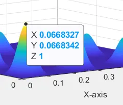
x=0.06683 ,y=0.06683, z=1
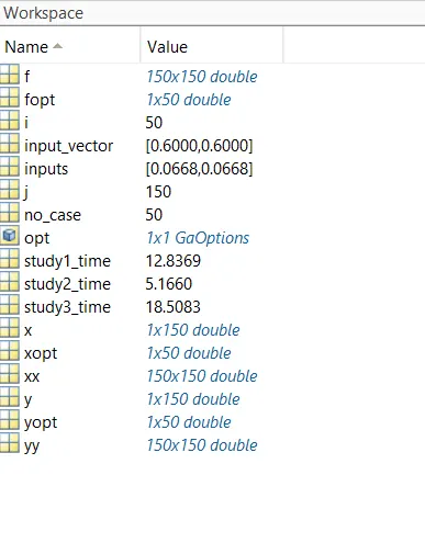
Workspace value
ERRORS
No major errors were faced during coding only some variable issues.
REFERENCE
https://in.mathworks.com/help/matlab/random-number-generation.html
https://www.sciencedirect.com/topics/engineering/genetic-algorithmhttps://www.sciencedirect.com/topics/engineering/genetic-algorithm