Rankine cycle Simulator

AIM: To create a Rankine Cycle Simulator using MATLAB.

OBJECTIVE:

1. To calculate the state points of the Rankine Cycle based on user inputs. 
2. To calculate the  Network output and Back work ratio.
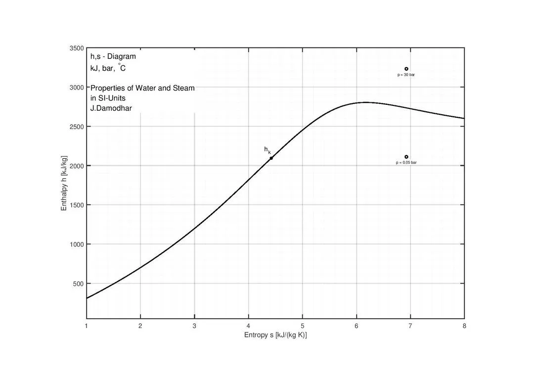
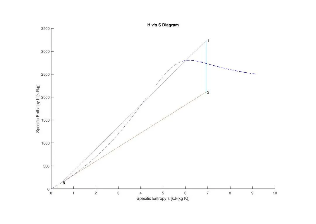
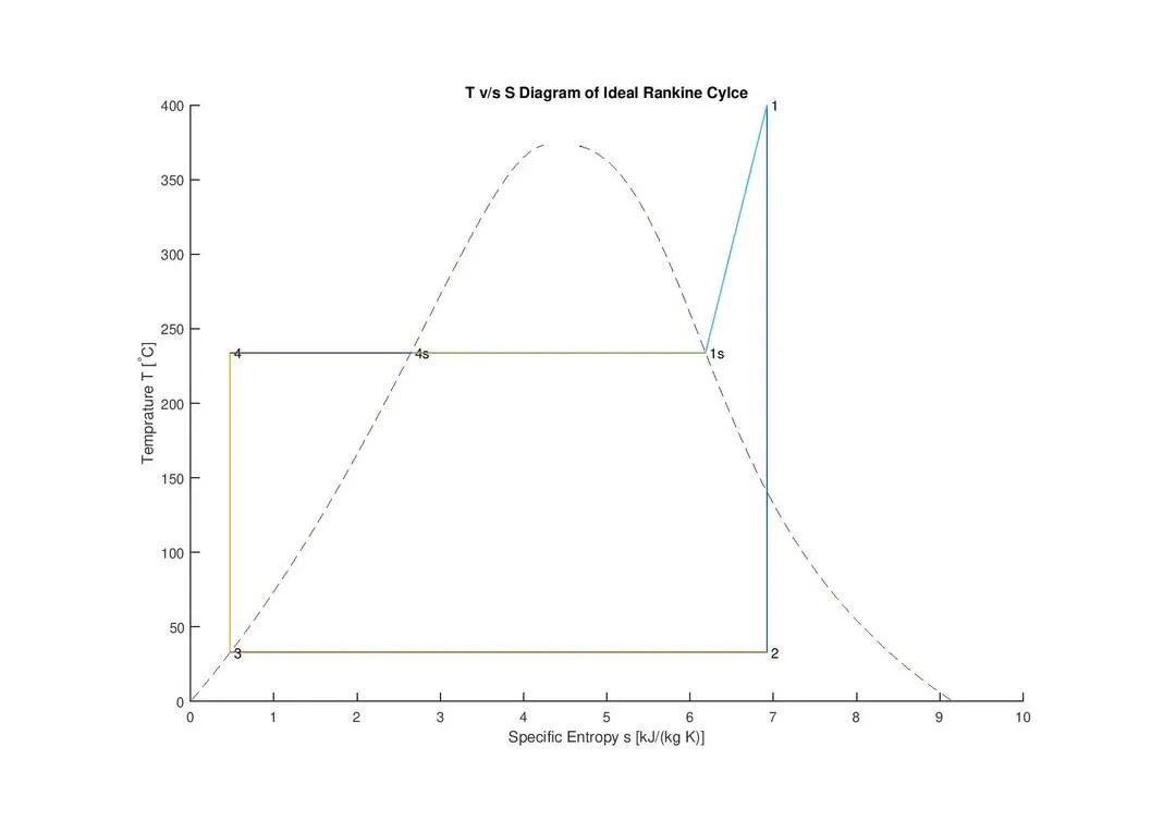
3. To plot the corresponding T-s and h-s plots for the given set of inputs.

THEORY :

The Rankine cycle is the fundamental operating cycle of all power plants where an operating fluid is continuously evaporated and condensed. The selection of operating fluid depends mainly on the available temperature range. The figure shows the idealized Rankine cycle.

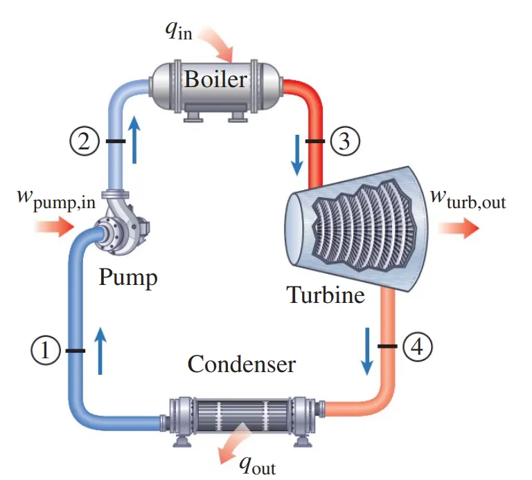
The ideal cycle for vapor power plants. 

The ideal Rankine cycle does not involve any internal irreversibilities and consists of the following four processes:
1-2 Isentropic compression in a pump
2-3 Constant pressure heat addition in a boiler
3-4 Isentropic expansion in a turbine
4-1 Constant pressure heat rejection in a condenser

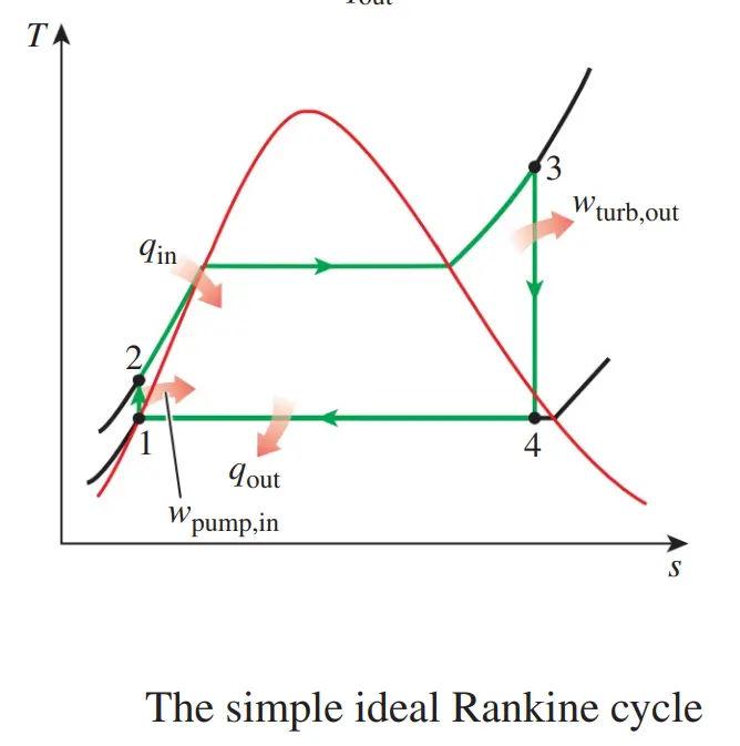
Water enters the pump at state 1 as saturated liquid and is compressed isentropically to the operating pressure of the boiler. The water temperature increases somewhat during this isentropic compression process due to a slight decrease in the specific volume of water. The vertical distance between states 1 and 2 on the T-s diagram is greatly exaggerated for clarity.

W_P= H₂ – H_{1 ,}

Water enters the boiler as a compressed liquid at state 2 and leaves as superheated vapor at state 3. The boiler is basically a large heat exchanger where the heat originating from combustion gases, nuclear reactors, or other sources is transferred to the water essentially at constant pressure. The boiler, together with the section where the steam is superheated (the superheater), is often called the steam generator.

_{Qin = H3 – H2  ,}

 The superheated vapor at state 3 enters the turbine, where it expands isentropically and produces work by rotating the shaft connected to an electric generator.

_{Wt = H3– H4 ,}

The pressure and the temperature of the steam drop during this process to the values at state 4, where steam enters the condenser. At this state, steam is usually a saturated liquid-vapor mixture with high quality. Steam is condensed at constant pressure in the condenser, which is basically a large heat exchanger, by rejecting heat to a cooling medium such as a lake, a river, or
the atmosphere

_{Qout = H4 – H1,}

GOVERNING EQUATIONS :

1. Wnet = Wt - Wp
2. ηthemal = (Wnet/Qin)*100
3. Steam rate (SSC)= 3600/Wt
4. Back work ratio (BWR)= (Wp/Wt)*100

main code Rankine_cycle

clc
close all 
clearvars

% T     Temperature (°C)
% p	    Pressure    (bar)
% h	    Enthalpy    (kJ/kg)
% v	    Specific volume (m3/kg)
% s	    Specific entropy (kJ/kg-K)

f1 = fopen('Rankine_cycle.txt','w');

% Rankine cycle 
fprintf(f1,'ttt! RANKINE CYCLE STIMULATOR !nttt ^^^^^^^^*^^^^^*^^^^^^^^^^^ n');
% processure in rankine cycle
fprintf(f1,'tCycle,nt 1-2 is Isentropic Expansion in the Turbine');
fprintf(f1,'nt 2-3 is Constant Pressure heat rejection by the Condenser');
fprintf(f1,'nt 3-4 is Isentropic Compression in the Pump');
fprintf(f1,'nt 4-1 is Constant Pressure heat addition by the BoilerntHere,');
fprintf(f1,'nt T     Temperature t(°C)');
fprintf(f1,'nt P	   Pressure    t(bar)');
fprintf(f1,'nt H	   Enthalpy    t(kJ/kg)');
fprintf(f1,'nt S	   Specific entropyt(kJ/kg-K)n ');
% inputs for rankine cycle
i = 1;
p(1,1) = input('Enter the Pressure at the Turbine Inlet (in Bar) : ');
p(4,1) = p(1,1);
fprintf(f1,'n %i)Enter the Pressure at the Turbine Inlet (in Bar)tt: %4i Bar',i,p(1,1));
i = i+1;
p(2,1) = input('Enter the Pressure at the Condenser (in Bar) : ');
p(3,1) = p(2,1);
fprintf(f1,'n %i)Enter the Pressure at the Condenser (in Bar)ttt: %4.2f Bar',i,p(2,1));
i = i+1;
t(1,1) = input('Enter the Temperature at the Turbine inlet (in °C) : ');
fprintf(f1,'n %i)Enter the Temperature at the Turbine inlet (in °C)t: %4.0f °Cn',i,t(1,1));

% computation function
% At state point 1 :
% h1
t(1,1);                                 % t1
p(1,1);                                 % p1
s(1,1) = XSteam('s_pt',p(1,1),t(1,1));  % s1
h(1,1) = XSteam('h_pt',p(1,1),t(1,1));  % h1
% done

% At state point 2 :
% h2
p(2,1);                            % p2
s(2,1) = s(1,1);                   % s2
sf2 = XSteam('sL_P',p(2,1));
sg2 = XSteam('sV_P',p(2,1));
hf2 = XSteam('hL_P',p(2,1));
hg2 = XSteam('hV_P',p(2,1));
x2 = ((s(2,1)-sf2)/(sg2-sf2));     % x2
h(2,1) = hf2+(x2*(hg2-hf2));       % h2
%done 

% At state point 3 :
% hf3
hf3 = XSteam('HL_P',p(2,1));        % h3
h(3,1) = hf3;
sf3 = XSteam('sL_P',p(2,1));        % s3
s(3,1) = sf3;
t(3,1) = XSteam('t_ps',p(2,1),s(3,1)); % t3
t(2,1) = t(3,1);                    % t2
p(3,1);                             % p3
% done

% At state point 4 :
% hf4
p(4,1);                             % p4
s(4,1) = sf3;                       % s4
vf2 = XSteam('vL_p',p(3,1));
Wp = vf2*(p(1,1)-p(2,1))*100;       %  Pump work (Wp)
hf4 = hf3 + Wp;                     
h(4,1) = hf4;                       % h4
t(4,1) = XSteam('Tsat_p',p(4,1));
% for Boiler heat addition (Q1)
% hf4 + Q1 = h1
Qin = h(1,1) - hf4;

% for Turbine work (Wt)
% h1 = Wt + h2
Wt = abs(h(2,1) - h(1,1));

% for Condenser heat rejection (Q2)
% h2 = Q2 + h4


% for Pump work (Wp)
% hf3 + Wp = hf4


% out put
Wnet = Wt - Wp;             % Net work 
Nthem = (Wnet/Qin)*100;     % ηthemal
s_s_c = 3600/Wt;            % Specific Steam Consumption
B_W_R = (Wp/Wt)*100;        % Back-work ratio

% out put print
fprintf(f1,'ntt  ! State Points !ntt   ^^^^^^*^^^^^^^');
for i = 1:4
   fprintf(f1,'nt At State point %d :',i);
   fprintf(f1,'n|t P%d : %4.2f   Bartt|',i,p(i,1));
   fprintf(f1,'n|t T%d : %5.3f  °Ctt|',i,t(i,1));
   fprintf(f1,'n|t H%d : %6.2f kJ/kgtt|',i,h(i,1));
   fprintf(f1,'n|t S%d : %3.2f    kJ/kg-Kt|',i,s(i,1));
   if i==2
       fprintf(f1,'n|t X%d : %3.2f    ttt|',i,x2);
   end
   fprintf(f1,'n');
end

fprintf(f1,'nntt  ! FINAL RESULTS !ntt   ^^^^^^*^^^^^^^^');
fprintf(f1,'n|t 1)Turbine Work    : %6.2f kJ/kgt|',Wt);
fprintf(f1,'n|t 2)Pump work       : %4.2f   kJ/kgt|',Wp);
fprintf(f1,'n|t 3)Net workdone    : %5.2f  kJ/kgt|',Wnet);
fprintf(f1,'n|t 4)ηthemal         : %2.2f percentaget|',Nthem);
fprintf(f1,'n|t 5)Back-work ratio : %5.3f percentage t|',B_W_R);
fprintf(f1,'n|t 6)Specific Steam Consumption : %3.2f kg/kWh  |',s_s_c);
fprintf(f1,'n|*******************The End**********************|');


% T v/s S diagram
% Calculation for plotting Liquid and Vapour lines 
% 
% <>
% 
temp = linspace(1, 373, 500);
for i = 1 : length(temp)
     H_L(i) = XSteam('hL_T', temp(i));
     H_V(i) = XSteam('hV_T', temp(i));
     S_L(i) = XSteam('sL_T', temp(i));
     S_V(i) = XSteam('sV_T', temp(i));
end

% T v/s S diagram

S1 = s(1,1);
S2 = s(2,1);
S2g = XSteam('sV_p',p(2,1));
S2f = XSteam('SL_p',p(2,1));
S3 = s(3,1);
S4 = s(4,1);
S1f = XSteam('SL_p',p(1,1));
S1g = XSteam('sV_p',p(1,1));
T1 = t(1,1);
T2 = t(2,1);
T2s = XSteam('Tsat_p',p(2,1));
T3 = t(3,1);
T4 = t(4,1);
T1s = XSteam('Tsat_p',p(1,1));
H1 = h(1,1);
H2 = h(2,1);
H3 = h(3,1);
H4 = h(4,1);
figure(1) % T-S
hold on
plot([S1 S2], [T1 T2])
text(S1,T1,' 1')
text(S2,T2,' 2')

plot([S2 S3], [T2 T3])
text(S3,T3,' 3')
plot([S3 S4], [T3 T4])
text(S4,T4,' 4')
plot([S4 S1f], [T4 T1s])
text(S1f,T1s,' 4s')
plot([S1f S1g], [T1s T1s])
text(S1g,T1s,' 1s')
plot([S1g S1], [T1s T1])
plot(S_L, temp, 'b', 'linestyle','--')
plot(S_V, temp, 'b', 'linestyle','--')

title('T v/s S Diagram of Ideal Rankine Cylce')
ylabel('Temprature T [^circ{}C]')
xlabel('Specific Entropy s [kJ/(kg K)]')
  %%%%%%%%%%%%%%%%%%%%%%%%%%%%%%%%%%%%%%%%%%%%%%%%%%%%%%%%%%%%%%%%%%%%%%%%%%%%
  % PRINT
  %%%%%%%%%%%%%%%%%%%%%%%%%%%%%%%%%%%%%%%%%%%%%%%%%%%%%%%%%%%%%%%%%%%%%%%%%%%%
  % settingt to print a .pdf copy

  filename = ['T-s-Diagram01_' date];
  paper_offset = 0.5; % centimeters

    set(gcf,'PaperType','A4','PaperOrientation','Landscape')
    paper = get(gcf,'PaperSize');
    paper_pos = [paper_offset paper_offset paper(1)-2*paper_offset ...
                 paper(2)-2*paper_offset];
    set(gcf,'PaperPosition',paper_pos)
    print(gcf,'-dpdf',filename)
% h v/s S diagram
figure(2) 
hold on
plot([S1 S2], [H1 H2]);
text(S1,H1,' 1')
plot([S2 S3], [H2 H3]);
text(S2,H2,' 2')
plot([S3 S4], [H3 H4]);
text(S3,H3,' 3')
plot([S4 S1], [H4 H1]);
text(S4,H4,' 4')
plot(S_L, H_L, 'b','linestyle','--')
plot(S_V, H_V, 'b','linestyle','--')      
title('H v/s S Diagram')
ylabel('Specific Enthalpy h [kJ/kg]')
xlabel('Specific Entropy s [kJ/(kg K)]')
  %%%%%%%%%%%%%%%%%%%%%%%%%%%%%%%%%%%%%%%%%%%%%%%%%%%%%%%%%%%%%%%%%%%%%%%%%%%%
  % PRINT
  %%%%%%%%%%%%%%%%%%%%%%%%%%%%%%%%%%%%%%%%%%%%%%%%%%%%%%%%%%%%%%%%%%%%%%%%%%%%
  % settingt to print a .pdf copy

filename = ['h-s-Diagram01_' date];
  paper_offset = 0.5; % centimeters

    set(gcf,'PaperType','A4','PaperOrientation','Landscape')
    paper = get(gcf,'PaperSize');
    paper_pos = [paper_offset paper_offset paper(1)-2*paper_offset ...
                 paper(2)-2*paper_offset];
    set(gcf,'PaperPosition',paper_pos)
    print(gcf,'-dpdf',filename)
  
% h v/s S diagram
[~,~] = thermo_diagram_plot('hs',p,s,'MultiplePoints','On','WetSteamArea','On','Legend','on','XLim',[1 8],'YLim',[50 3500]);
hold on
 
% T v/s S diagram
[~,~] = thermo_diagram_plot('Ts',p,'WetSteamArea','On','VaporFractions','off','Legend','on','XLim',[1 8],'YLim',[25 450]);

fclose(f1); 

Function code: thermo_diagram_plot

which is standard code from

https://in.mathworks.com/matlabcentral/fileexchange/24903-diagrams-of-thermodynamic-state-of-water

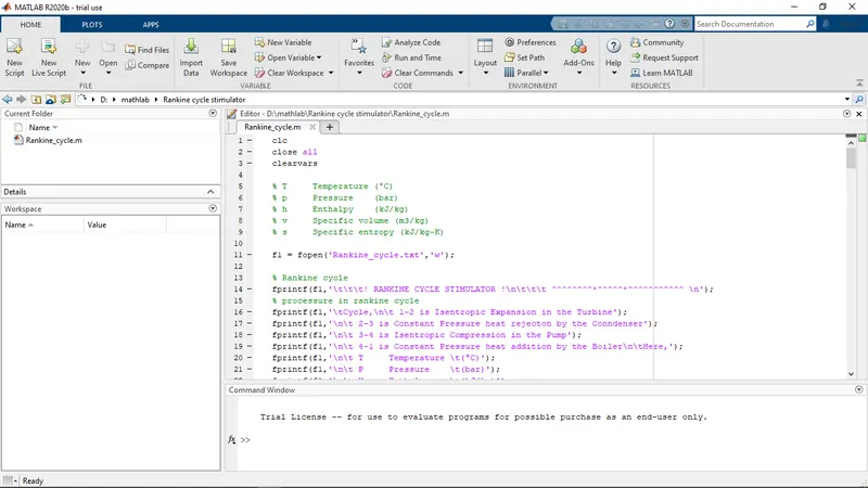
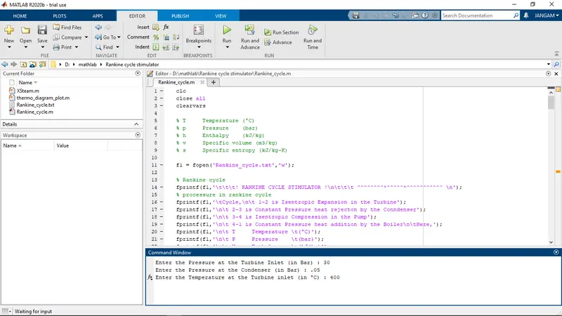
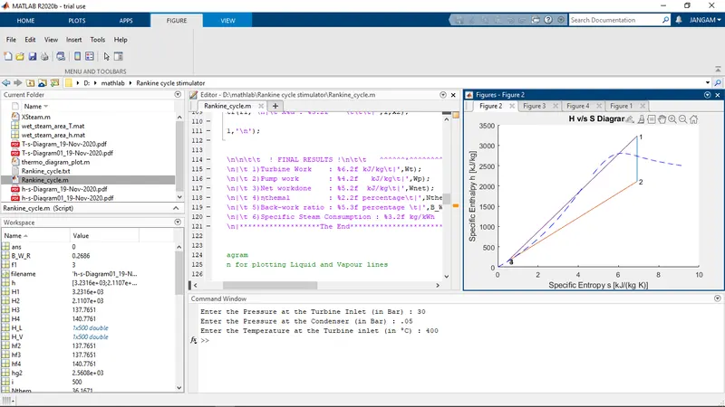
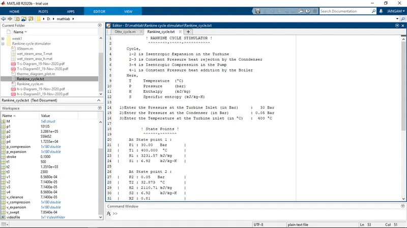
output saved as in .txt file

! RANKINE CYCLE STIMULATOR!
^^^^^^^^*^^^^^*^^^^^^^^^^^
RANKINE Cycle,
1-2 is Isentropic Expansion in the Turbine
2-3 is Constant Pressure heat rejection by the Condenser
3-4 is Isentropic Compression in the Pump
4-1 is Constant Pressure heat addition by the Boiler
Here,
T Temperature (°C)
P Pressure (bar)
H Enthalpy (kJ/kg)
S Specific entropy (kJ/kg-K)

1)Enter the Pressure at the Turbine Inlet (in Bar): 30 Bar
2)Enter the Pressure at the Condenser (in Bar): 0.05 Bar
3)Enter the Temperature at the Turbine inlet (in °C): 400 °C

! State Points!
^^^^^^*^^^^^^^
At State point 1 :
| P1 : 30.00 Bar |
| T1 : 400.000 °C |
| H1 : 3231.57 kJ/kg |
| S1 : 6.92 kJ/kg-K |

At State point 2 :
| P2 : 0.05 Bar |
| T2 : 32.873 °C |
| H2 : 2110.71 kJ/kg |
| S2 : 6.92 kJ/kg-K |
| X2 : 0.81 |

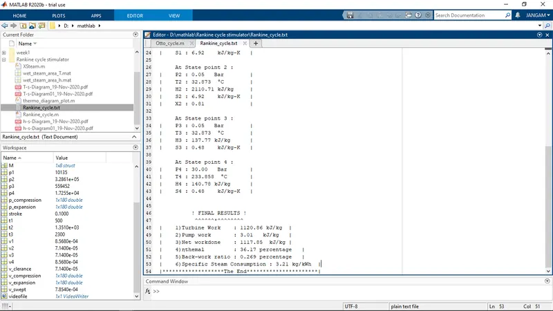
At State point 3 :
| P3 : 0.05 Bar |
| T3 : 32.873 °C |
| H3 : 137.77 kJ/kg |
| S3 : 0.48 kJ/kg-K |

At State point 4 :
| P4 : 30.00 Bar |
| T4 : 233.858 °C |
| H4 : 140.78 kJ/kg |
| S4 : 0.48 kJ/kg-K |

! FINAL RESULTS!
^^^^^^*^^^^^^^^
| 1)Turbine Work : 1120.86 kJ/kg |
| 2)Pump work : 3.01 kJ/kg |
| 3)Net workdone : 1117.85 kJ/kg |
| 4)ηthemal : 36.17 percentage |
| 5)Back-work ratio : 0.269 percentage |
| 6)Specific Steam Consumption : 3.21 kg/kWh |
|*******************The End**********************|

 Screenshort of outps

ploted graph

1. T - S graph through standard code

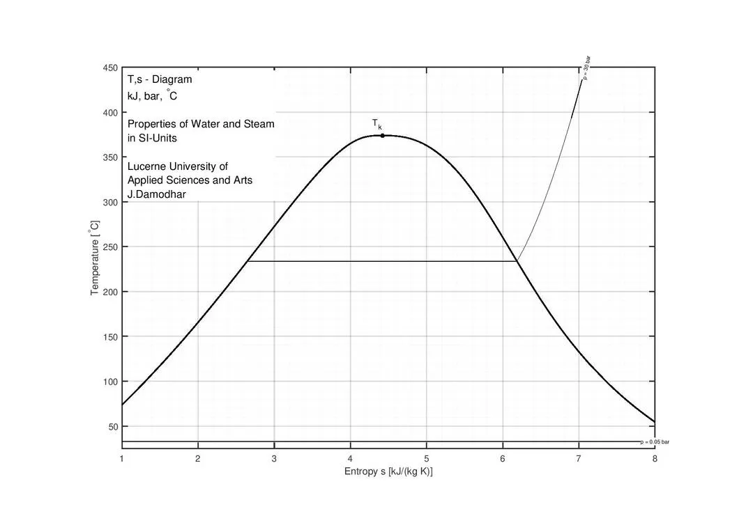
2. T - S graph through standard code:

1. H - S graph:

1. T - S graph:

Conclusion:

1. The T-S and H-S performance curves of the Rankine Cycle were plotted.
2. Values at each state are computed
3. Performance parameters are determined as below
    Turbine Work: 1120.86 kJ/kg   
    Pump work: 3.01 kJ/kg          
    Network done: 1117.85 kJ/kg  
    ηthemal: 36.17 % 
    Back-work ratio : 0.2 %
    Specific Steam Consumption : 3.21 kg/kWh 

REFERENCES : 

1. THERMODYNAMICS: AN ENGINEERING APPROACH, EIGHTH EDITION--YUNUS A.  ÇENGEL & MICHAEL A. BOLES

2.  https://in.mathworks.com/matlabcentral/fileexchange/24903-diagrams-of-thermodynamic-state-of-water