pipe flow simulation with an inlet Reynolds number of 100,1000 and 10,000

Aim: To run a pipe flow simulation with an inlet Reynolds number of 100, 1000 & 10000.

Theory:

Reynolds Number:

It is a ratio of inertial forces to the viscous forces within a fluid

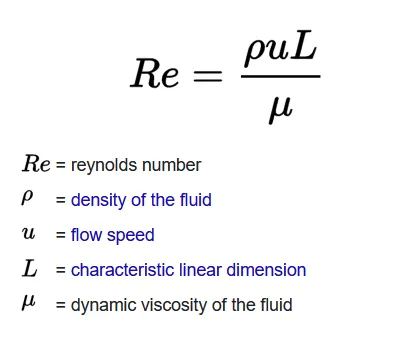
• In our case
  • the characteristic length is the diameter of the pipe which is 0.05m
  • the density of the fluid is 1000 kg/m^3
  • dynamic viscosity is 1.002*10^-3 Pa.s
• To create the flow simulation for different Reynolds numbers we must prescribe the boundary conditions with velocity as a parameter. So, using the Reynolds number formula for each Reynolds number we would get the corresponding velocity which can be prescribed as a boundary condition to create a flow simulation.
• For the diameter of 0.05m, the corresponding velocities are as follows
  • For Re = 100 the velocity U = 0.002004 m/s
  • For Re = 1000 the velocity U = 0.02004 m/s
  • For Re = 10000 the velocity U = 0.2004 m/s

Procedure:

• Firstly, I started by creating a pipe geometry with a diameter of 0.05m.
• After creating the geometry by using the lids I created the closed structure on both sides of the pipe.
• Then I created a new project in the flow simulation module.
• All the input data according to the problem statement are selected and saved the data.
• I have used 3 different boundary conditions to describe the flow of the pipe
  • Velocity at the inlet
  • Static pressure at the exit
  • Wall for the length of the pipe
• I have created 3 different line probes at the exit of the pipe
• I have created XY plots between these line probes and the velocity at the inlet
• I have created a cut plot at the exit of the pipe which represents the velocity profile of the flow.
• Finally, I have created a parametric study using the above base study for different velocities that I have calculated for different Reynolds numbers.

Results:

1. line probes at 95%, 90%, and 85% of the pipe length.

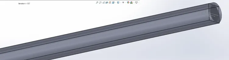
The line probes are prescribed at the exit at the required position along the pipeline.

2. Compare the normalized velocity profile at each of these locations

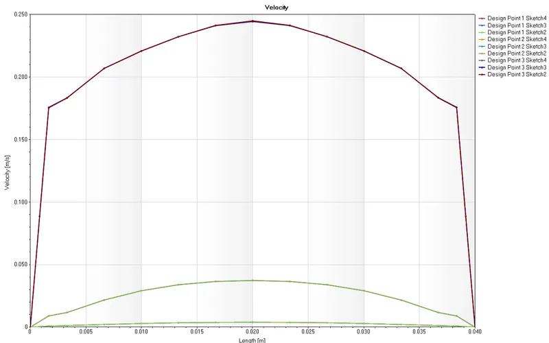
This plot represents the velocity profile at each location of the line probes. This parabolic curve represents the boundary layer formation at the different probe lines.

3. Normalize the velocity profile by the inlet velocity.

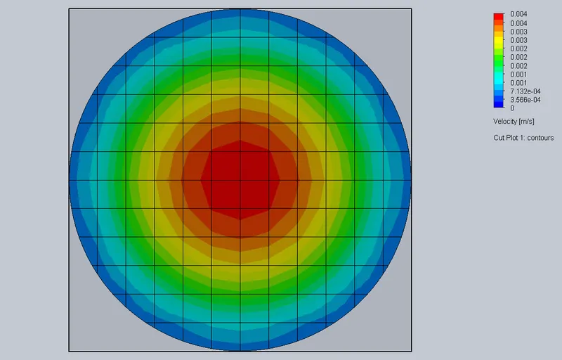
Velocity normal to the face (Inlet velocity) = 0.002004m/s

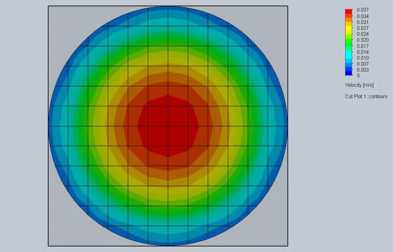
Velocity normal to the face (Inlet velocity) = 0.02004m/s

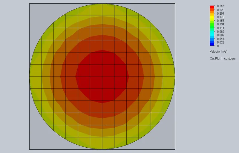
Velocity normal to the face (Inlet velocity) = 0.2004m/s

The above pictures depict the velocity profile at the end of the pipe. For different Reynolds numbers, we have different velocity profiles. From the figure it is clear that the flow has a max velocity at the center of the pipe and the velocity decreases as we move away from the center of the pipe, depicting the boundary layer formation.