Curvefit using MATLAB
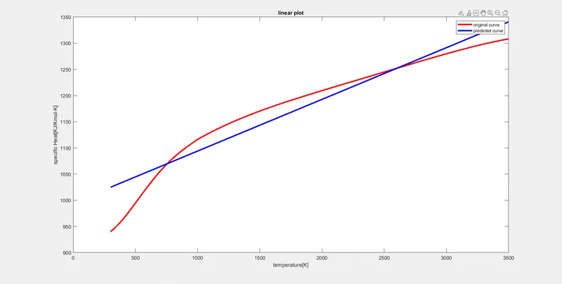
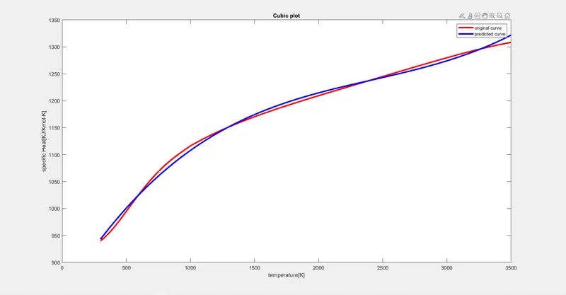
Aim: To write a MATLAB program to fit a linear and cubic polynomial for the Cp data.
Governing Equation and Data
The curve fit is a technique of finding an algebraic expression that best fits the given data.
Here we will find the coefficients of different orders of the equation:
y = ax+b
y = ax^2+bx+c
y = ax^3+bx^2+cx+d
The flow of the project
1.Code and explanation to fit linear polynomial for the Cp data.
2.Code and explanation to fit cubic polynomial for the Cp data.
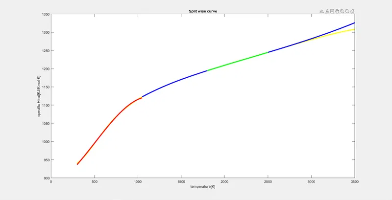
3.Code showing split-wise method.
4.Results.
1.Code and explanation to fit linear polynomial for the Cp data.
clear all
close all
clc
%preparing the data
cp_data = load('data');
temperature = cp_data(:,1);
cp = cp_data(:,2);
%data for predicted cp
coeff = polyfit(temperature,cp,1);
predicted_cp = polyval(coeff,temperature);
%original plot
plot(temperature, cp,'linewidth',3,'color','r')
hold on
%curvefitting plot
plot(temperature,predicted_cp,'linewidth',3,'color','b')
2.Code and explanation to fit cubic polynomial for the Cp data.
clear all
close all
clc
%preparing the data
cp_data = load('data');
temperature = cp_data(:,1);
cp = cp_data(:,2);
%data for predicted cp
coeff = polyfit(temperature,cp,3);
predicted_cp = polyval(coeff,temperature);
%original plot
plot(temperature, cp,'linewidth',3,'color','r')
hold on
%curvefitting plot
plot(temperature,predicted_cp,'linewidth',3,'color','b')
3.Code showing split-wise method.
clear all
close all
clc
%preparing the data
cp_data = load('data');
temperature = cp_data(:,1);
cp = cp_data(:,2);
%Data1
x1 = temperature(1:750);
y1 = cp(1:750);
%Data2
x2 = temperature(751:1500);
y2 = cp(751:1500);
%Data3
x3 = temperature(1501:2200);
y3 = cp(1501:2200);
%DATA4
x4 = temperature(2201:3200);
y4 = cp(2201:3200);
%%CURVE FIT
%cp = a*T^2+b*T+c
%coeff & predected cp values of data1
C1= polyfit(x1,y1,2);
Cp1 = polyval(C1,x1);
%coeff & predected cp values of data2
C2 = polyfit(x2,y2,2);
Cp2 = polyval(C2,x2);
%coeff & predected cp values of data3
C3 = polyfit(x3,y3,2);
Cp3 = polyval(C3,x3);
%coeff & predected cp values of data4
C4 = polyfit(x4,y4,2);
Cp4 = polyval(C3,x4);
%Comparing my curve fit with original data
plot(temperature,cp,'linewidth',3,'color','y')
xlabel('temperature[K]')
ylabel('specific Heat[KJ/Kmol-K]')
hold on
plot(x1,Cp1,'linewidth',3,'color','r');
plot(x2,Cp2,'linewidth',3,'color','b');
plot(x3,Cp3,'linewidth',3,'color','g');
plot(x4,Cp4,'linewidth',3,'color','m');
3.Code explanation:
*firstly load the data to the program by using the load command.
*Assigning the variables (temperature, cp) to the data gives us the desired values of the data.
*Using the plot command plot the data.
*By using the polyfit command we can find the coefficients of the desired order of equations and by using polyval we can get the predicted cp values by using the coefficients we have found.
*Now plotting this data and the temp gives us the curve with which we can compare the curve with the original curve.
1.How to make the curve fit perfectly?
The perfect fit means the predicted curve should be the same as the original one without any slightest deflection. To make the curve fit perfectly we need to minimize the errors. This can be done by using a split-wise method which is shown in the above program.
2.How to get the best fit?
The best fit of the curve is determined by the following parameters
1.The sum of squares due to error (SSE).
2.R-Square.
3.Adjusted R-square.
4.Root mean square error.
3.what could be done to improve the cubic bit?
This can be done by splitting the data into various sets and finding the curve fit for the individual set where we will get the best fit with fewer errors
Results