Week 2 Air standard Cycle

Aim: To write a code to solve an otto cycle and create plots of pv diagram and calculate the termal efficiency of otto cycle.

Governing Equation:

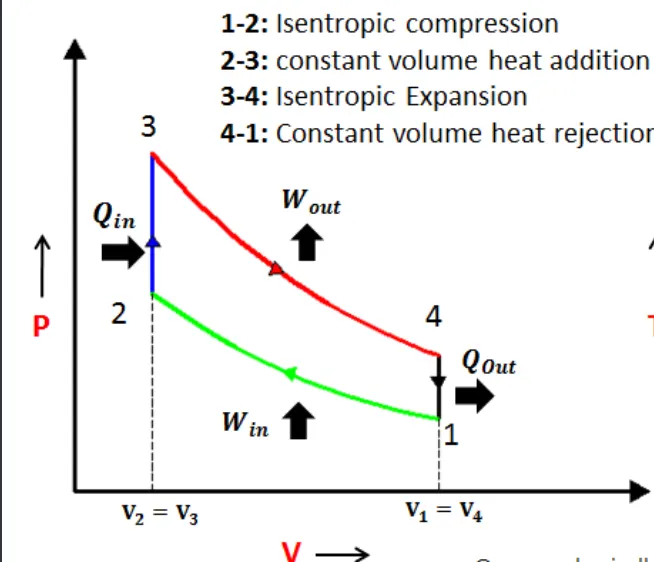
two stroke engines operates on the otto cycle.

for isentropic process 1-2 & 3-4

p1v1^gamma = p2v2^gamma

for process 2-3 & 4-1

p1v1/t1 = p2v2/t2

change of volume inside the combustion chamber is given by = 1+0.5(cr-1)[R+1-cos(theta)-((R^2-sin(theta))^2]

Flow of the project

1. Code to solve an otto cycle and to draw a pv diagram.
2. Code explaination.
3. results

1.Code to solve an otto cycle and to draw a PV diagram:

import math

import matplotlib.pyplot as plt

#engine dimensions

bore = 0.1

stroke = 0.1

con_rod = 0.15

g = 1.4

cr = 8

def enginekinematics(bore,stroke,con_rod,cr,start_crank,end_crank):

a = stroke/2

R = con_rod/a

#volume computation

v_s = (math.pi/4)*pow(bore,2)*stroke

v_c = v_s/(cr-1)

sc = math.radians(start_crank)

ec = math.radians(end_crank)

numvalues =100

dtheta = (ec-sc)/(numvalues-1)

v = []

for i in range(0,numvalues):

theta = sc + i*dtheta

term1 = 0.5*(cr-1)

term2 = R +1 -math.cos(theta)

term3 = pow(R,2) -pow(math.sin(theta),2)

term3 = pow(term3,0.5)

v.append((1 +term1*(term2-term3))*v_c)

return v

#volume computation

v_s = (math.pi/4)*pow(bore,2)*stroke

v_c = v_s/(cr-1)

# state point 1

p1 = 101325

t1 = 500

v1 = v_s +v_c

#state point 2

#p1v1^g = p2v2^g \ p1v1/t1 = p2v2/t2

v2 = v_c

p2 = p1*(v1/v2)**g

t2 = p2*v2*t1/p1*v1

const = p1*pow(v1,g)

v_compression = enginekinematics(bore,stroke,con_rod,cr,180,0)

p_compression=[]

for v in v_compression:

p_compression.append(const/pow(v,g))

#state point 3

v3 = v2

t3 = 3000

p3 = (p2*v2*t3)/(v3*t2)

#state point 4

v4 = v1

p4 = p3*pow(v3,g)/pow(v4,g)

const1 = p3*pow(v3,g)

v_expansion = enginekinematics(bore,stroke,con_rod,cr,0,180)

p_expansion=[]

for v in v_expansion:

p_expansion.append(const1/pow(v,g))

#thermal efficiency

t_eff = 1-(1/pow(cr,(g-1)))

print(t_eff)

plt.plot(v_compression,p_compression)

plt.plot([v2,v3],[p2,p3])

plt.plot(v_expansion,p_expansion)

plt.plot([v1,v4],[p1,p4])

plt.show()

2.code explanation:

• Initiate the code by importing the libraries required to run the program.
• Give the engine dimensions such as bore, stroke, length of the con rod.
• Using the command “def” we will create a function that consists of the engine dimensions as inputs for running the function.
• Using the formula given we can get the volumes for both compression stroke and expansion stroke.
• We will then compute the pressure and volume at each state point.
• Finally, by using the “plt.plot” command, we will plot all the points at each state point which will give us the otto cycle.
• Finally, the thermal efficiency of the otto cycle is calculated.

Results

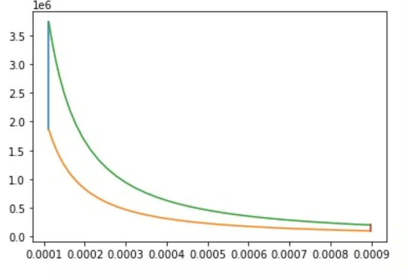
thermal efficiency of the otto cycle: